Genome contamination Analysis
This is an R Markdown Notebook for Quality Check and contamination analysis in genome assembly projects. We use GenomeScope and Blobtools programs to check the quality of the our data and our genome assemblies.
What is blobtools?
Is “A modular command-line solution for visualisation, quality control and taxonomic partitioning of genome dataset” (https://github.com/DRL/blobtools) (Challis et al. 2020).
Preparing files for blobtools
First, we blast our genome assemblies to know nt databases (eg. NCBI) using blastn program (2.X, Altschul et al. X ).
# /bin/sh
# ----------------Parameters---------------------- #
#$  -S /bin/sh
#$ -pe mthread 12
#$ -q mThC.q
#$ -l mres=96G,h_data=8G,h_vmem=8G
#$ -cwd
#$ -j y
#$ -N acti_blast
#$ -o acti_blast.log
#$ -m bea
#$ -M solracarias@si.edu
#
# ----------------Modules------------------------- #
module load bioinformatics/blast
#
# ----------------Your Commands------------------- #
#
echo + `date` job $JOB_NAME started in $QUEUE with jobID=$JOB_ID on $HOSTNAME
echo + NSLOTS = $NSLOTS
blastn -db /data/genomics/db/ncbi/db/latest_v4/nt/nt -query HPA_04_pilon.fasta -outfmt "6 qseqid staxids bitscore std" -max_target_seqs 10 -max_hsps 1 -evalue 1e-20 -num_threads $NSLOTS -out HPA_blast.out
#
echo = `date` job $JOB_NAME done
Second, we map our raw reads sequences to our genome assembly. We used minimap2 to map reads and later we used samtools to convert from sam to bam and finally sort the bam file.
# /bin/sh
# ----------------Parameters---------------------- #
#$  -S /bin/sh
#$ -pe mthread 20
#$ -q mThM.q
#$ -l mres=96G,h_data=8G,h_vmem=8G,himem
#$ -cwd
#$ -j y
#$ -N acti_blast
#$ -o acti_blast.log
#$ -m bea
#$ -M solracarias@si.edu
#
# ----------------Modules------------------------- #
source ~/.bashrc
conda activate minimap2
module load bioinformatics/samtools/1.9
#
# ----------------Your Commands------------------- #
#
echo + `date` job $JOB_NAME started in $QUEUE with jobID=$JOB_ID on $HOSTNAME
echo + NSLOTS = $NSLOTS
minimap2 -ax map-hifi -t 20 /scratch/genomics/solracarias/Panama_geminant_project/c_atrilobata/chromis_atrilobata_hifiasm_asm_bp_p_ctg.fasta /scratch/stri_ap/solracarias_data/owen_fish_genomes_data/files.rc.byu.edu/owen_fish/22D/22D_ccs/m54336U_210226_220508.Q20.fastq | samtools sort -@20 -O BAM -o c_atriolobata_mapped.bam -
  #
  echo = `date` job $JOB_NAME done
With bloobtools2 we create a database with Blast results (out file) and Mapped reads (sorted bam file).
qrsh -pe mthread 8
module load bio/blobtools/2.6.3
#Create a BlobDir
#blobtools create --fasta /scratch/genomics/solracarias/remy/blob/HPA_04_pilon.fasta HPA_04_pilon

blobtools create --fasta /scratch/genomics/solracarias/Panama_geminant_project/c_atrilobata/chromis_atrilobata_hifiasm_asm_bp_p_ctg.fasta c_atrilobata_blobt_nb

blobtools create --fasta /scratch/genomics/solracarias/Panama_geminant_project/c_cyanea/chromis_cyanea.asm.bp.p_ctg.fasta c_cyanea_blobtnb

blobtools create --fasta /scratch/genomics/solracarias/Panama_geminant_project/c_fulva/c_fulva_hifiasm.asm.bp.p_ctg.fa c_fulva_blobt_nb

blobtools create --fasta /scratch/genomics/solracarias/Panama_geminant_project/c_multilineata/chromis_multilineata.asm.bp.p_ctg.fasta  c_multilineata_blobt_nb

blobtools create --fasta /scratch/genomics/solracarias/Panama_geminant_project/p_colonus/p_colonus_hifiasm.asm.bp.p_ctg.fa p_colonus_blobt_nb

blobtools create --fasta /scratch/genomics/solracarias/Panama_geminant_project/p_furcifer/paranthias_furcifer_hifiasm.asm.bp.p_ctg.fa p_furcifer_blobt_nb

blobtools create --fasta /scratch/genomics/solracarias/Panama_geminant_project/A_troshelii/A_troshelli_hifiasm.asm.bp.p_ctg.fa  a_troshelii_blobt_nb

#Add BLAST hits
blobtools add --threads 8 --hits /scratch/genomics/solracarias/Panama_geminant_project/c_atrilobata/c_atrilobata_blast.out --taxrule bestsumorder --taxdump /scratch/genomics/solracarias/remy/blob/blopbtools2_run/taxdump c_atrilobata_blobt_nb

blobtools add --threads 8 --hits /scratch/genomics/solracarias/Panama_geminant_project/c_cyanea/c_cyanea_blast.out --taxrule bestsumorder --taxdump /scratch/genomics/solracarias/remy/blob/blopbtools2_run/taxdump c_cyanea_blobtnb

blobtools add --threads 8 --hits /scratch/genomics/solracarias/Panama_geminant_project/c_fulva/c_fulva_blast.out  --taxrule bestsumorder --taxdump /scratch/genomics/solracarias/remy/blob/blopbtools2_run/taxdump c_fulva_blobt_nb

blobtools add --threads 8 --hits /scratch/genomics/solracarias/Panama_geminant_project/c_multilineata/c_multilineata_blast.out --taxrule bestsumorder --taxdump /scratch/genomics/solracarias/remy/blob/blopbtools2_run/taxdump c_multilineata_blobt_nb

blobtools add --threads 8 --hits /scratch/genomics/solracarias/Panama_geminant_project/p_colonus/p_colonus_blast.out --taxrule bestsumorder --taxdump /scratch/genomics/solracarias/remy/blob/blopbtools2_run/taxdump p_colonus_blobt_nb

blobtools add --threads 8 --hits /scratch/genomics/solracarias/Panama_geminant_project/p_furcifer/p_furcifer_blast.out --taxrule bestsumorder --taxdump /scratch/genomics/solracarias/remy/blob/blopbtools2_run/taxdump p_furcifer_blobt_nb

blobtools add --threads 8 --hits /scratch/genomics/solracarias/Panama_geminant_project/A_troshelii/a_troshelii_blast.out --taxrule bestsumorder --taxdump /scratch/genomics/solracarias/remy/blob/blopbtools2_run/taxdump a_troshelii_blobt_nb

#Add mapping coverage
blobtools add --threads 8 --cov /scratch/genomics/solracarias/Panama_geminant_project/c_atrilobata/c_atriolobata_mapped.bam c_atrilobata_blobt_nb

blobtools add --threads 8 --cov /scratch/genomics/solracarias/Panama_geminant_project/c_cyanea/c_cyanea_mapped.bam c_cyanea_blobtnb

blobtools add --threads 8 --cov /scratch/genomics/solracarias/Panama_geminant_project/c_fulva/c_fulva_mapped.bam c_fulva_blobt_nb

blobtools add --threads 8 --cov /scratch/genomics/solracarias/Panama_geminant_project/c_multilineata/c_multilineata_mapped.bam c_multilineata_blobt_nb

blobtools add --threads 8 --cov /scratch/genomics/solracarias/Panama_geminant_project/p_colonus/p_colonus_mapped.bam p_colonus_blobt_nb

blobtools add --threads 8 --cov /scratch/genomics/solracarias/Panama_geminant_project/p_furcifer/p_furcifer_mapped.bam  p_furcifer_blobt_nb

blobtools add --threads 8 --cov /scratch/genomics/solracarias/Panama_geminant_project/A_troshelii/a_troshelii_mapped.bam  a_troshelii_blobt_nb

##adding buscos
blobtools add --busco /scratch/genomics/solracarias/Panama_geminant_project/c_atrilobata/c_atrilobata_p1/run_actinopterygii_odb10/full_table.tsv c_atrilobata_blobt

blobtools add --busco /scratch/genomics/solracarias/Panama_geminant_project/c_cyanea/c_cyanea/run_actinopterygii_odb10/full_table.tsv  c_cyanea_blobt

blobtools add --busco /scratch/genomics/solracarias/Panama_geminant_project/c_fulva/c_fulva/run_actinopterygii_odb10/full_table.tsv  c_fulva_blobt

blobtools add --busco /scratch/stri_ap/solracarias_data/owen_fish_genomes_data/files.rc.byu.edu/owen_fish/GeAA28/ccs/chromis_multilineata_busco/run_actinopterygii_odb10/full_table.tsv c_multilineata_blobt

blobtools add --busco /scratch/genomics/solracarias/Panama_geminant_project/p_colonus/p_colonus/run_actinopterygii_odb10/full_table.tsv  p_colonus_blobt

blobtools add --busco /scratch/genomics/solracarias/Panama_geminant_project/p_furcifer/output_busco/p_furcifer/run_actinopterygii_odb10/full_table.tsv p_furcifer_blobt

#Download db  folder to desktop and run blobtools viewer

rclone copy blob_database  db3:hydra_backup/

  #Create interactive html page with the blobtools results. this command was run in my personal mac computer were I install blobtools2 using conda. remember to run this command from the folder where blobtools was install or make it to the PATH.

  #activate conda enviroment for blobtools2
  conda activate btk_env
./blobtools view --remote /Users/solracarias/Dropbox/de_contamination_geminate_panama/c_atrilobata_blobt/

  ./blobtools view --remote /Users/solracarias/Dropbox/de_contamination_geminate_panama/c_cyanea_blobt

./blobtools view --remote /Users/solracarias/Dropbox/de_contamination_geminate_panama/p_furcifer_blobt

./blobtools view --remote /Users/solracarias/Dropbox/de_contamination_geminate_panama/c_multilineata_blobt

./blobtools view --remote /Users/solracarias/Dropbox/de_contamination_geminate_panama/c_fulva_blobt

./blobtools view --remote /Users/solracarias/Dropbox/de_contamination_geminate_panama/c_atrilobata_blobt
You can play with viewer to change colors on figures, tables etc. Figures and tables can be downloaded and visualized.
Blobtools Results by fish species
Paranthias colonus
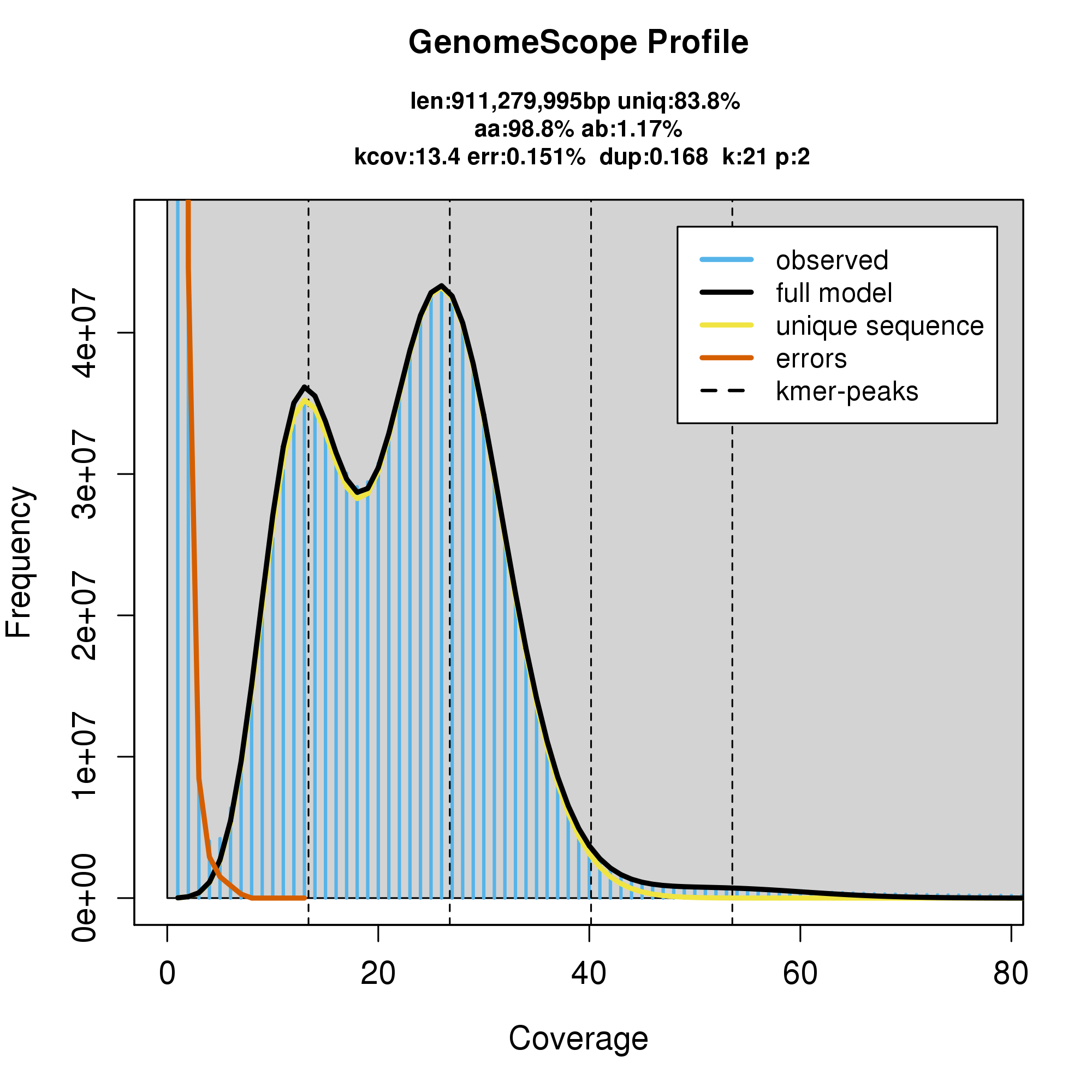
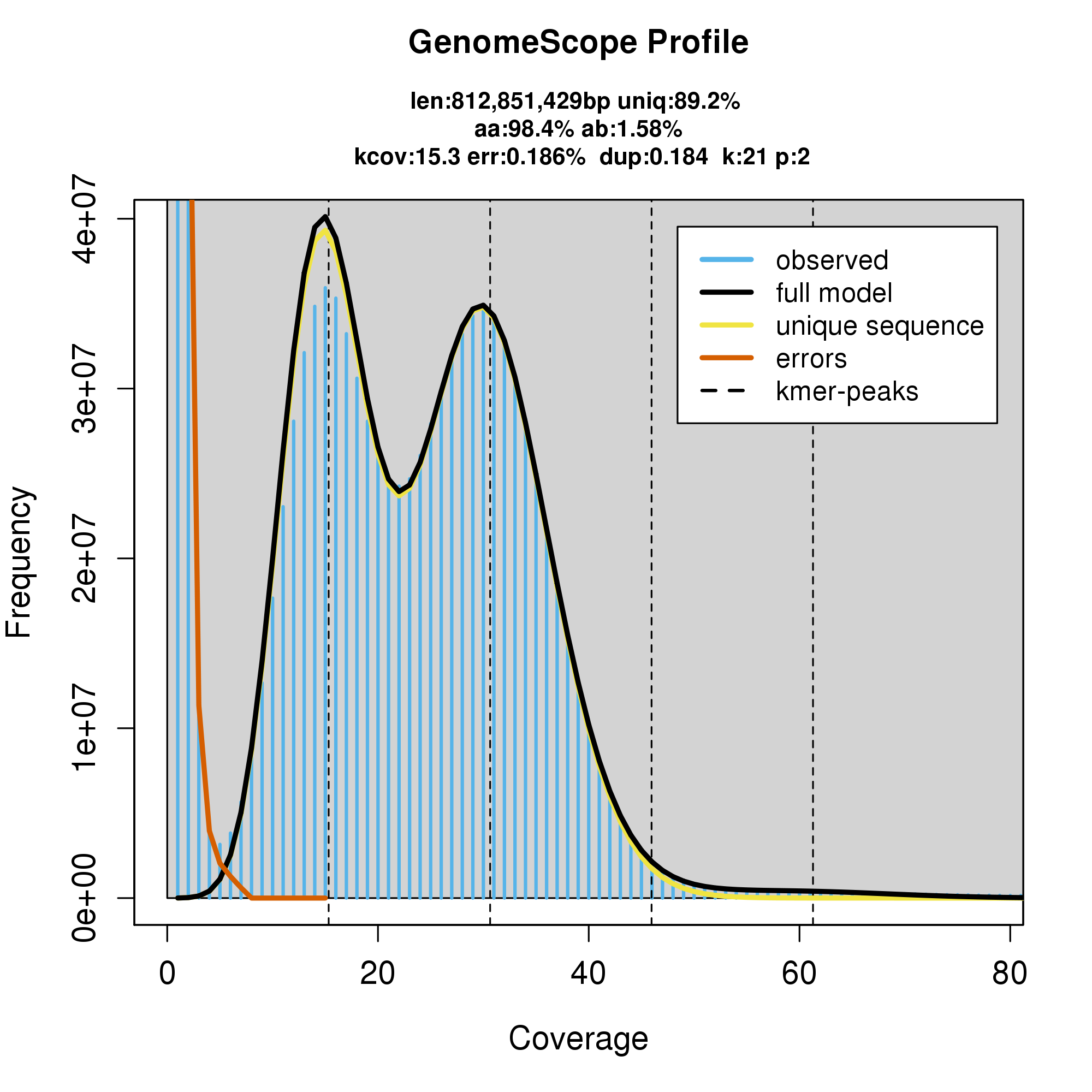
GenomeScope Results
#GenomeScope Resutls
knitr::include_graphics("p_colonus_blob_results/linear_plot.png")
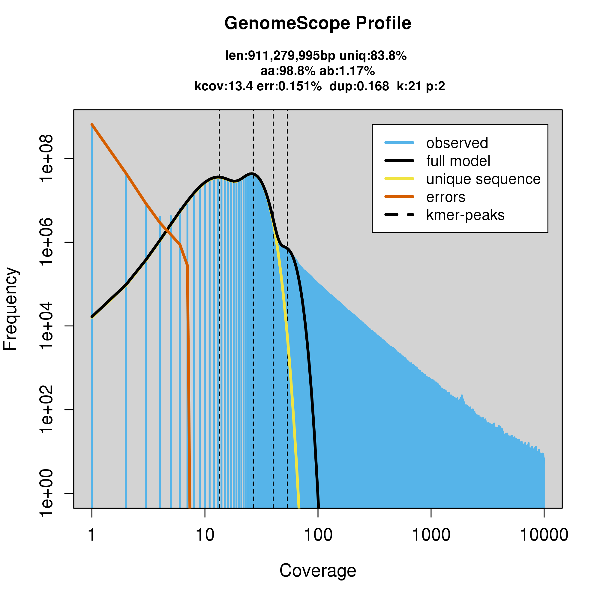
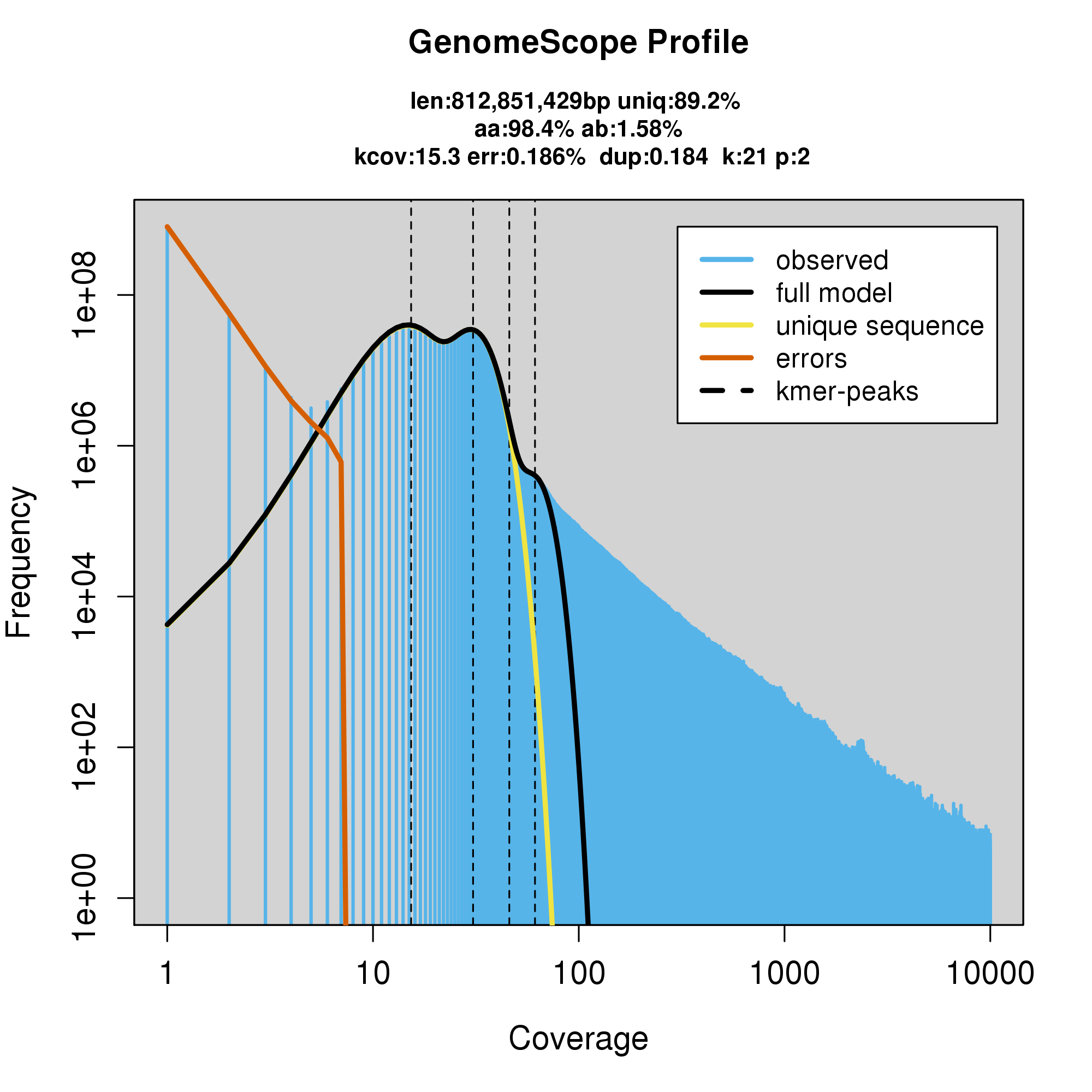
#GenomeScope Resutls
knitr::include_graphics("p_colonus_blob_results/log_plot.png")
Assembly statistics in a snail plot
knitr::include_graphics("p_colonus_blob_results/p_colonus_blobt_nb.snail.png")
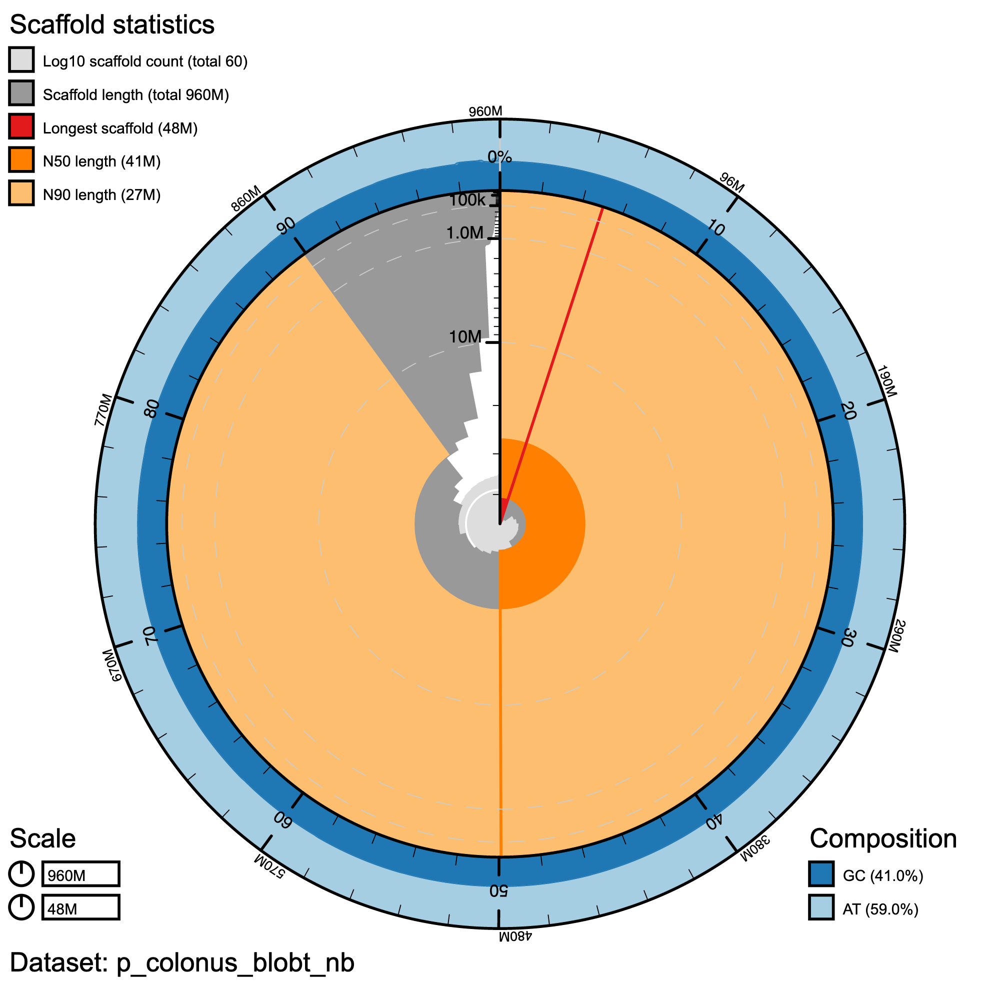
Snail plot summary of assembly statistics for P. colonus. The main plot is divided into 1,000 size-ordered bins around the circumference with each bin representing 0.1% of the 796,160,303 bp assembly. The distribution of record lengths is shown in dark grey with the plot radius scaled to the longest record present in the assembly (39,846,712 bp, shown in red). Orange and pale-orange arcs show the N50 and N90 record lengths (28,775,316 and 10,326,087 bp), respectively. The pale grey spiral shows the cumulative record count on a log scale with white scale lines showing successive orders of magnitude. The blue and pale-blue area around the outside of the plot shows the distribution of GC, AT and N percentages in the same bins as the inner plot.
Cumulative Plot
#cumulative plot
knitr::include_graphics("p_colonus_blob_results/p_colonus_blobt_nb.cumulative.png")
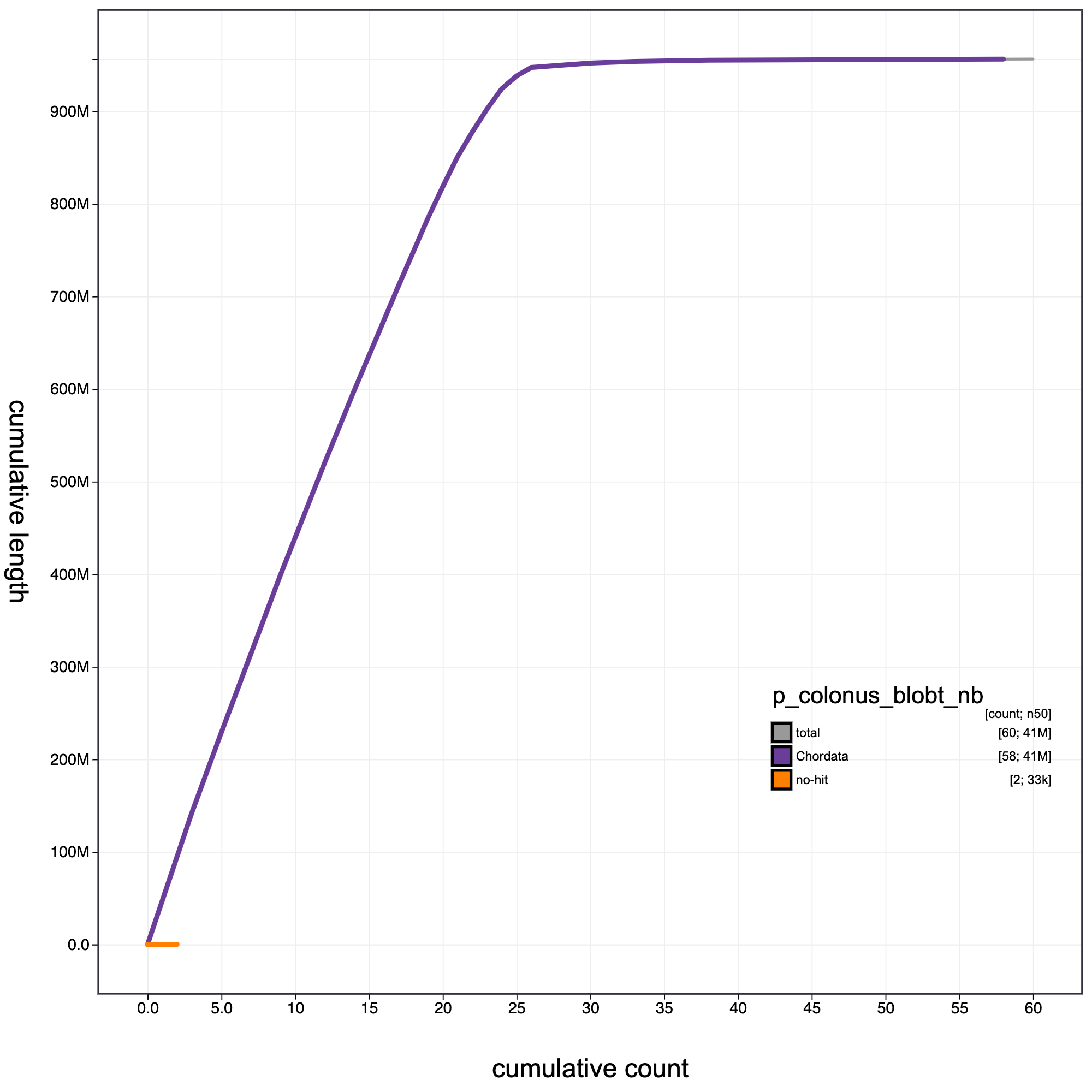
Cumulative record length for P. colonus. The grey line shows cumulative length for all records. Coloured lines show cumulative lengths of records assigned to each phylum using the bestsumorder taxrule.
blob plot
# blob plot
knitr::include_graphics("p_colonus_blob_results/p_colonus_blobt_nb.blob.circle.png")
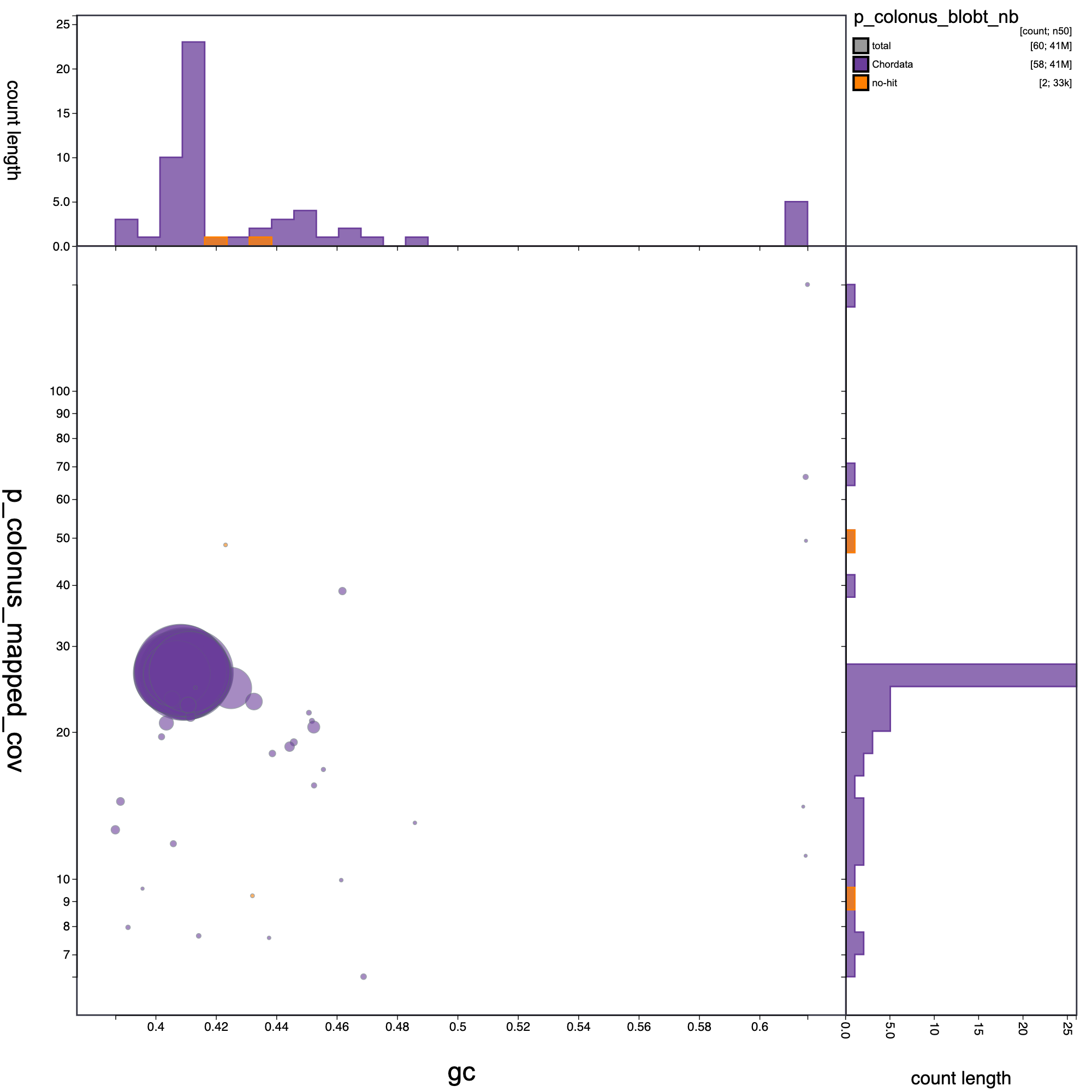
Blob plot of base coverage in a against GC proportion for records in assembly P. colonus. Records are coloured by phylum. Circles are sized in proportion to record length Histograms show the distribution of record length count along each axis.
blob table with varibles and categories
blob_results<- read.csv("p_colonus_blob_results/f6235d8a-0f0e-42b2-a6b8-2deeb62a6295.csv",header = T, sep = ",")
library(tidyverse)
blob_results<-select(blob_results, -1)
blob_results2<-select(blob_results, 1,8,2,3,7,4,5,6)
blob_results2<-select(blob_results2, -1)
#library(kableExtra)
#blob_results %>% kbl() %>% kable_styling()
library(DT)
options(scipen = 999)
datatable(blob_results2, rownames = FALSE, width = "100%", colnames = c("ID","GC","Length","Coverage","Phylum", "Class", "Family"),
          caption =
            htmltools::tags$caption(
              style = "caption-side: bottom; text-align: left;",
              "Table: ",
              htmltools::em("blob variables and Categories")),
          extensions = "Buttons",
          options = list(columnDefs =
                           list(list(className = "dt-left", targets = 0)),
                         dom = "Blfrtip", pageLength = 10,
                         lengthMenu = c(10, 20, 40, 70),
                         buttons = c("csv", "copy")))
Paranthias furcifer
GenomeScope Results
#GenomeScope Resutls
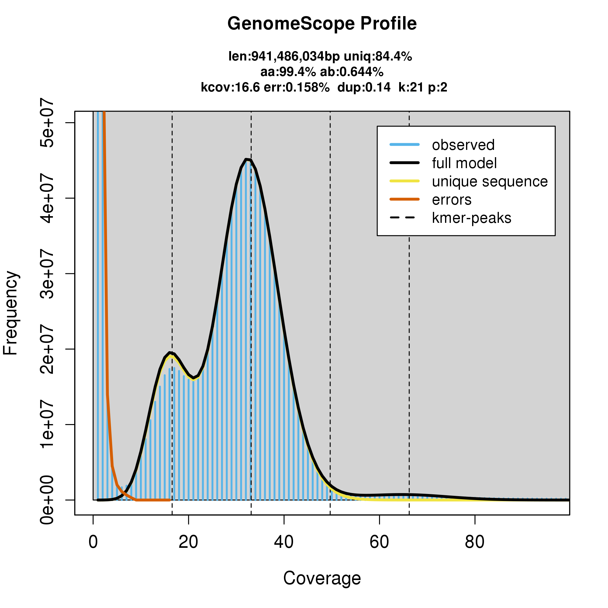
knitr::include_graphics("p_furcifer_blob_results/linear_plot.png")
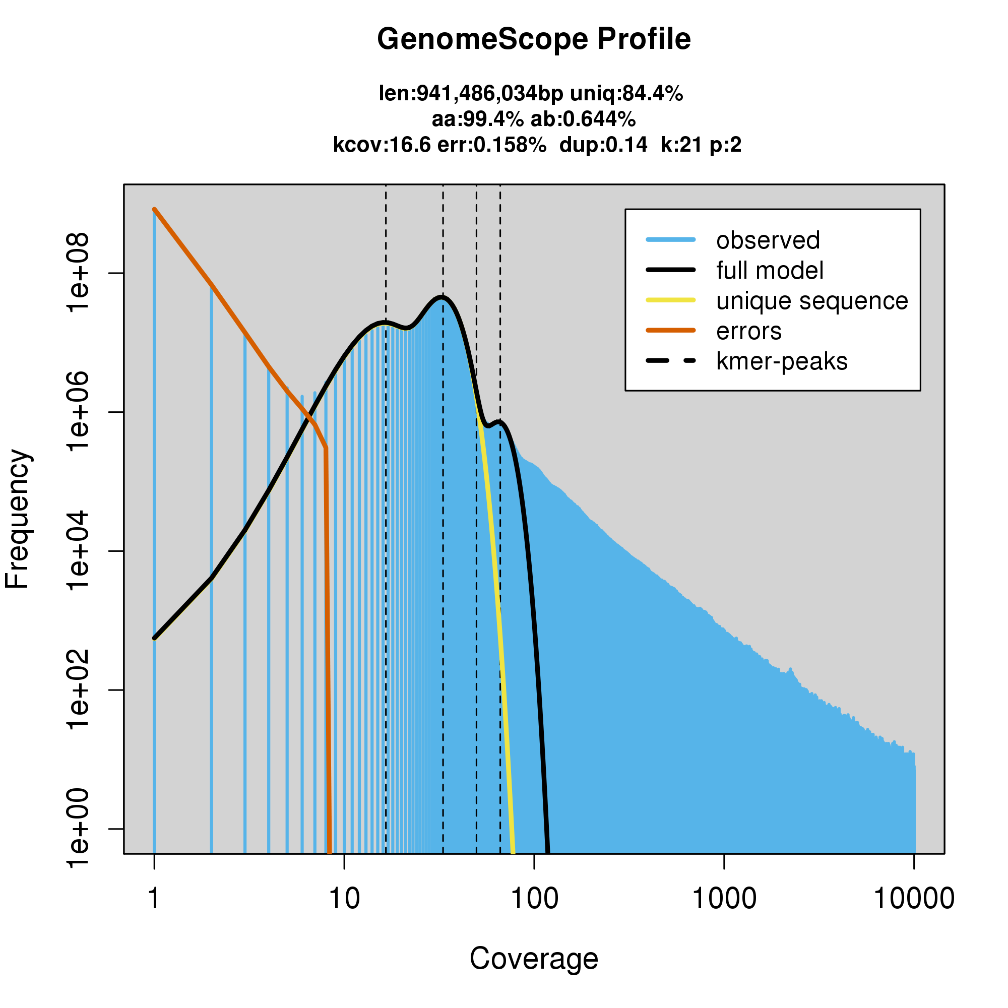
#GenomeScope Resutls
knitr::include_graphics("p_furcifer_blob_results/log_plot.png")
Assembly statistics in a snail plot
#Snail plot/
knitr::include_graphics("p_furcifer_blob_results/p_furcifer_blobt_nb.snail.png")
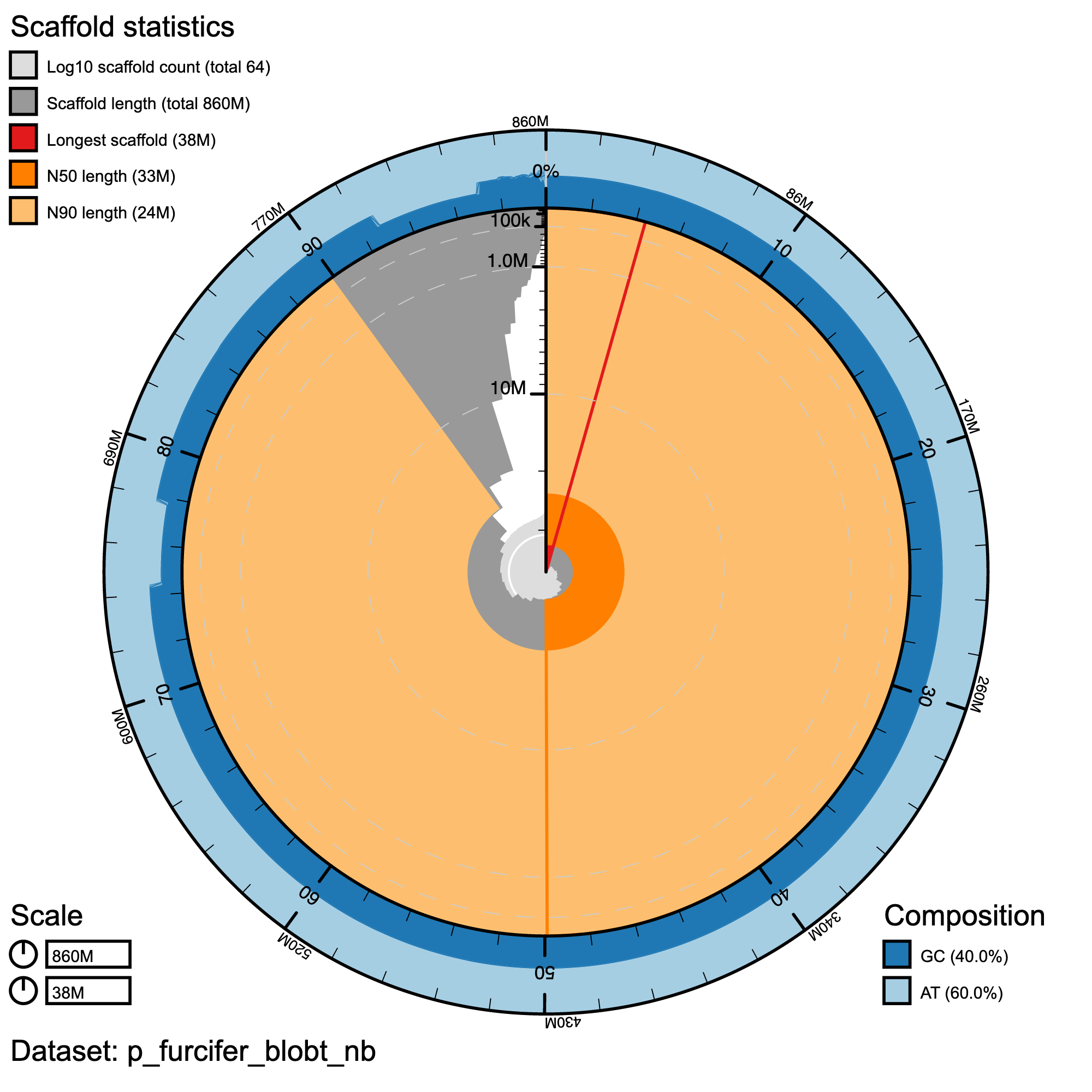
Snail plot summary of assembly statistics for P. furcifer.The main plot is divided into 1,000 size-ordered bins around the circumference with each bin representing 0.1% of the 860,147,216 bp assembly. The distribution of record lengths is shown in dark grey with the plot radius scaled to the longest record present in the assembly (38,289,793 bp, shown in red). Orange and pale-orange arcs show the N50 and N90 record lengths (32,505,010 and 23,558,019 bp), respectively. The pale grey spiral shows the cumulative record count on a log scale with white scale lines showing successive orders of magnitude. The blue and pale-blue area around the outside of the plot shows the distribution of GC, AT and N percentages in the same bins as the inner plot.
Cumulative Plot
#cumulative plot
knitr::include_graphics("p_furcifer_blob_results/p_furcifer_blobt_nb.cumulative.png")
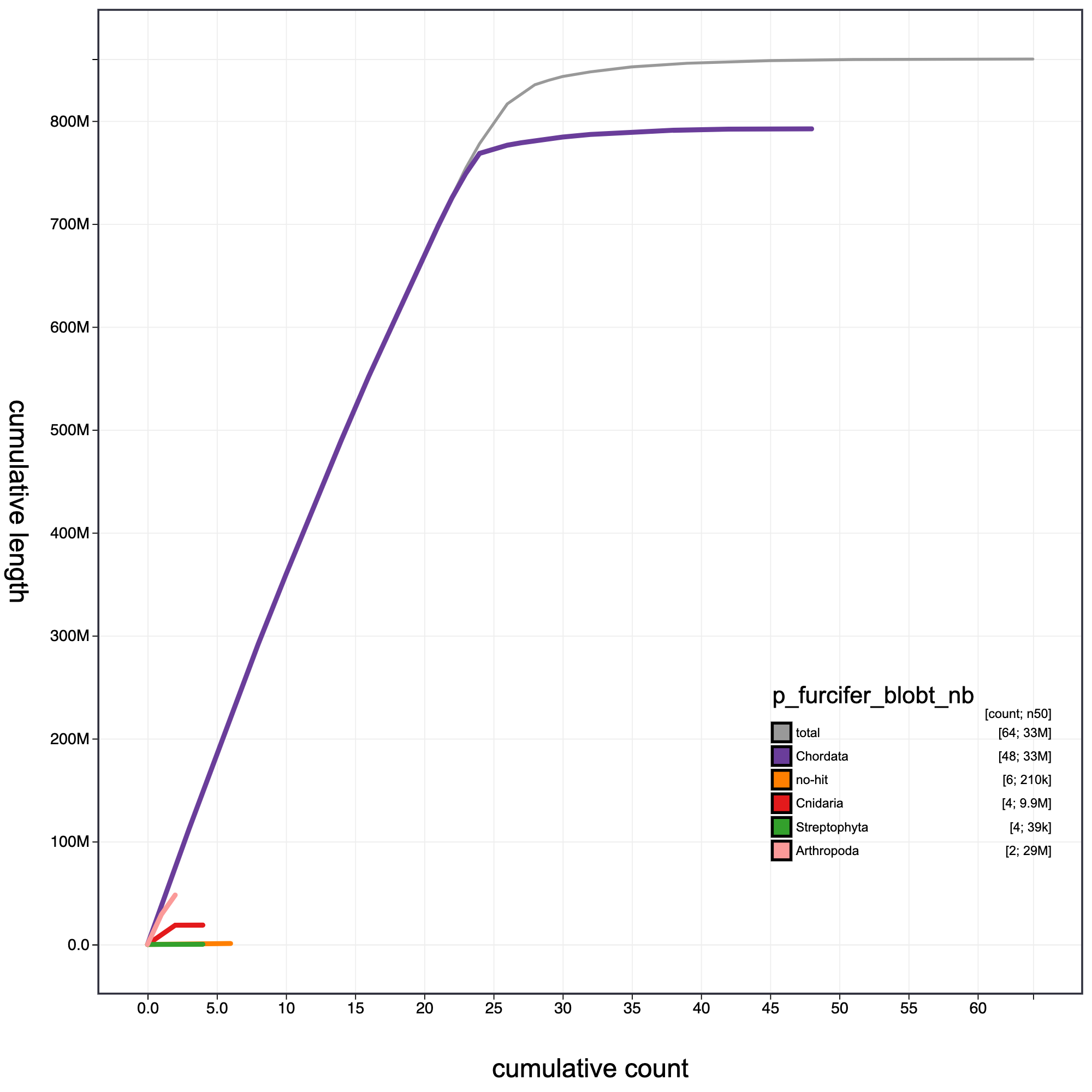
Cumulative record length for P. furcifer. The grey line shows cumulative length for all records. Coloured lines show cumulative lengths of records assigned to each phylum using the bestsumorder taxrule.
blob plot
# blob plot
knitr::include_graphics("p_furcifer_blob_results/p_furcifer_blobt_nb.blob.circle.png")
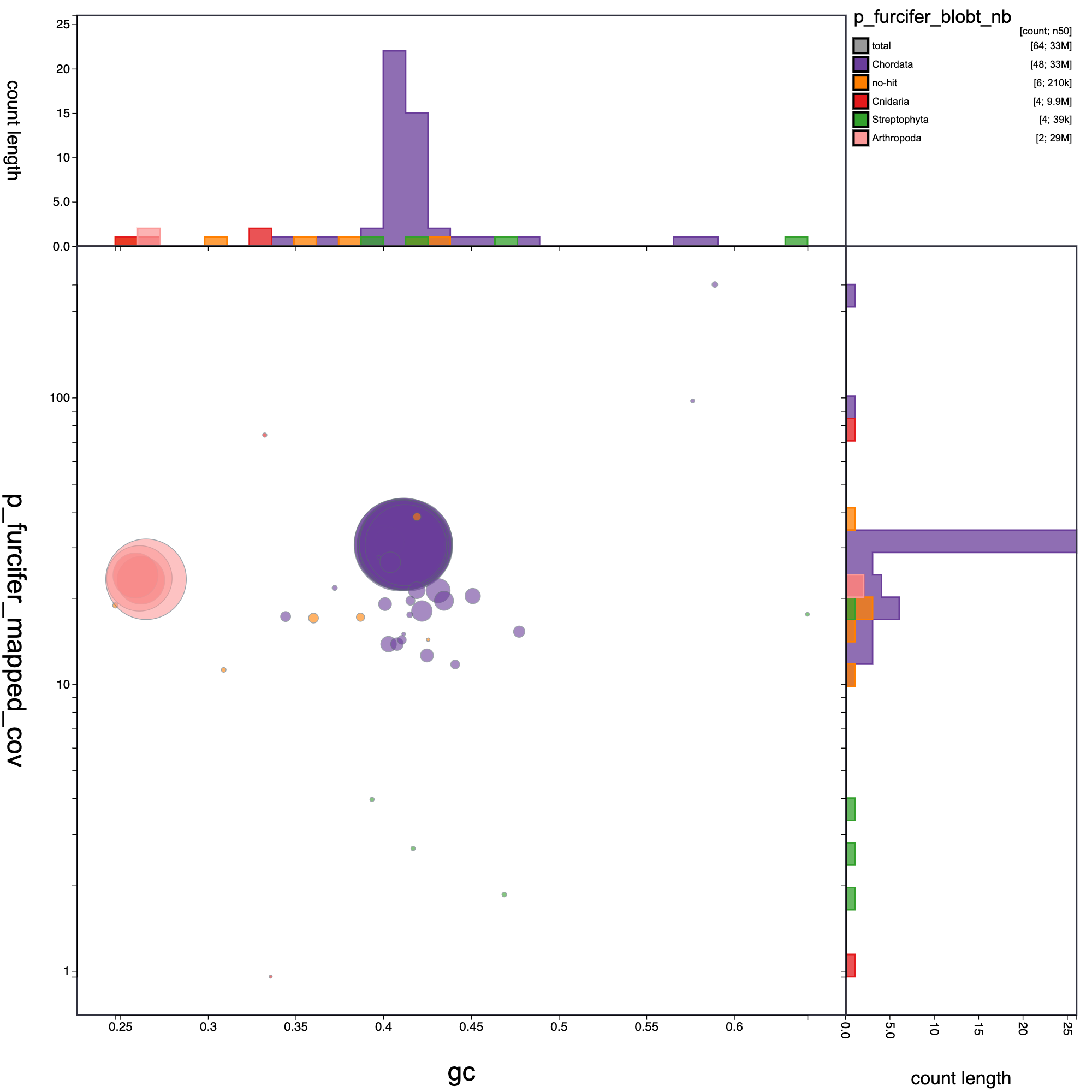
Blob plot of base coverage in p against GC proportion for records in P. furcifer assembly . Records are coloured by phylum. Circles are sized in proportion to record length Histograms show the distribution of record length sum along each axis.
blob table with varibles and categories
blob_results<- read.csv("p_furcifer_blob_results/7fc11af9-8af0-4b87-a060-df69dfa56242.csv",header = T, sep = ",")
library(tidyverse)
blob_results<-select(blob_results, -1)
blob_results2<-select(blob_results, 1,8,2,3,7,4,5,6)
blob_results2<-select(blob_results2, -1)
#library(kableExtra)
#blob_results %>% kbl() %>% kable_styling()
library(DT)
options(scipen = 999)
datatable(blob_results2, rownames = FALSE, width = "100%", colnames = c("ID","GC","Length","Coverage","Phylum", "Class", "Family"),
          caption =
            htmltools::tags$caption(
              style = "caption-side: bottom; text-align: left;",
              "Table: ",
              htmltools::em("blob variables and Categories")),
          extensions = "Buttons",
          options = list(columnDefs =
                           list(list(className = "dt-left", targets = 0)),
                         dom = "Blfrtip", pageLength = 10,
                         lengthMenu = c(10, 20, 40, 70),
                         buttons = c("csv", "copy")))
Cephalopholis fulva
GenomeScope Results
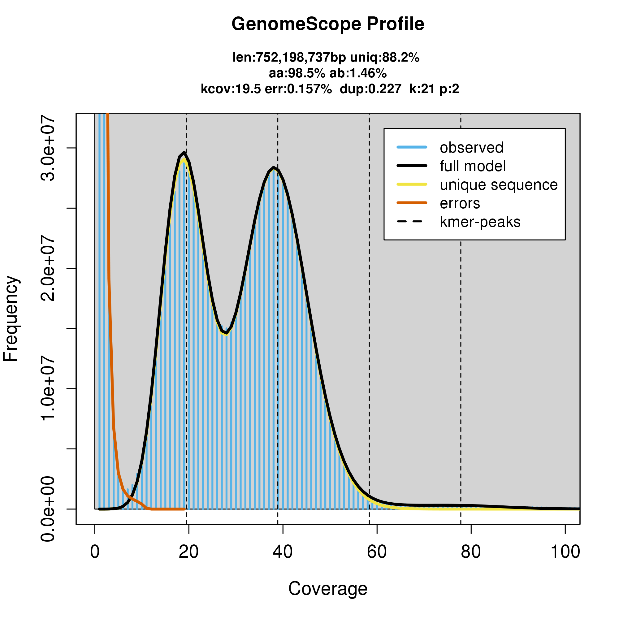
#GenomeScope Resutls
knitr::include_graphics("c_fulva_blob_results/linear_plot.png")
#GenomeScope Resutls
knitr::include_graphics("c_fulva_blob_results/log_plot.png")
Assembly statistics in a snail plot
#Snail plot/
knitr::include_graphics("c_fulva_blob_results/c_fulva_blobt_nb.snail.png")
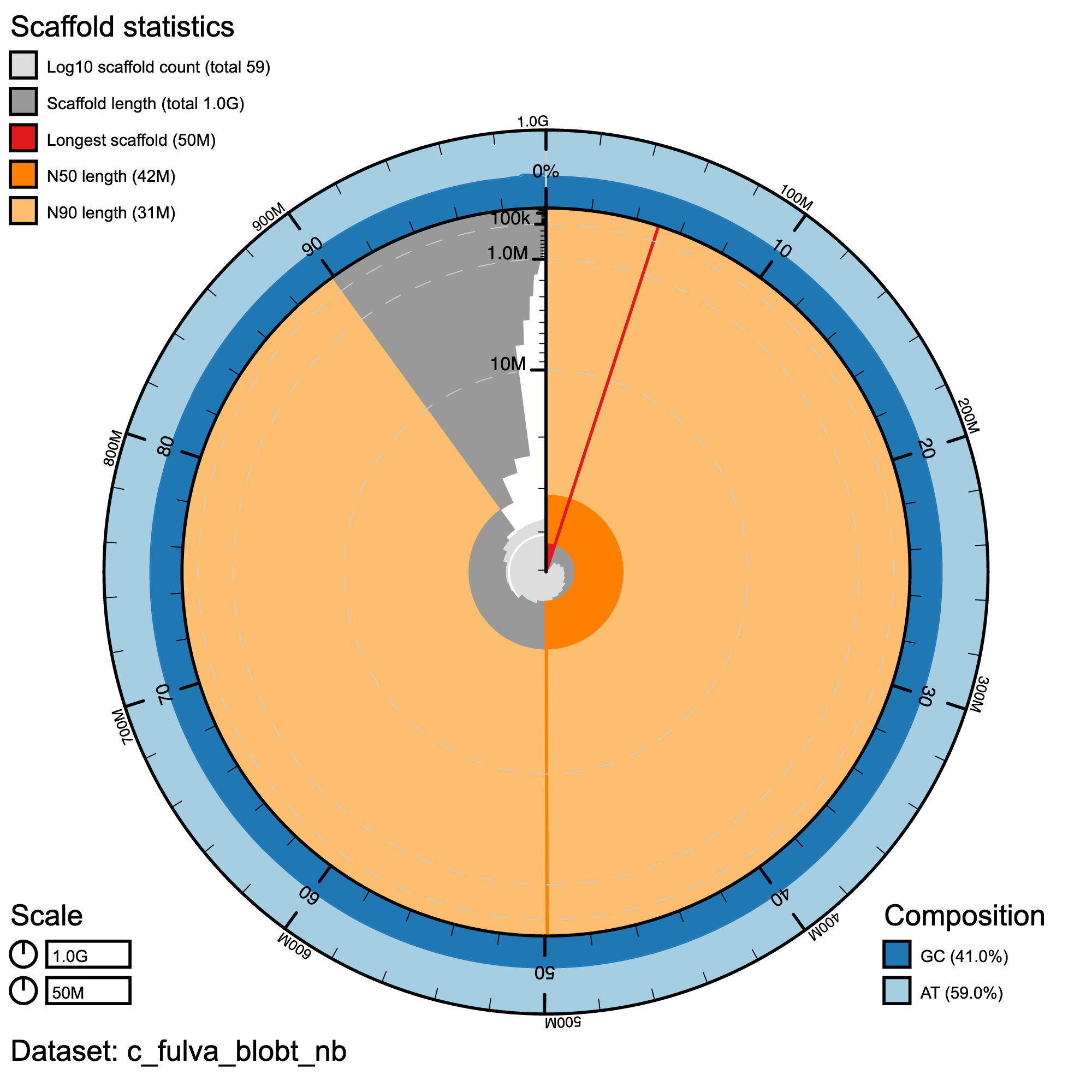
Snail plot summary of assembly statistics for C.fulva. The main plot is divided into 1,000 size-ordered bins around the circumference with each bin representing 0.1% of the 1,002,268,578 bp assembly. The distribution of record lengths is shown in dark grey with the plot radius scaled to the longest record present in the assembly (50,486,710 bp, shown in red). Orange and pale-orange arcs show the N50 and N90 record lengths (42,467,878 and 31,280,464 bp), respectively. The pale grey spiral shows the cumulative record count on a log scale with white scale lines showing successive orders of magnitude. The blue and pale-blue area around the outside of the plot shows the distribution of GC, AT and N percentages in the same bins as the inner plot.
Cumulative Plot
#cumulative plot
knitr::include_graphics("c_fulva_blob_results/c_fulva_blobt_nb.cumulative.png")
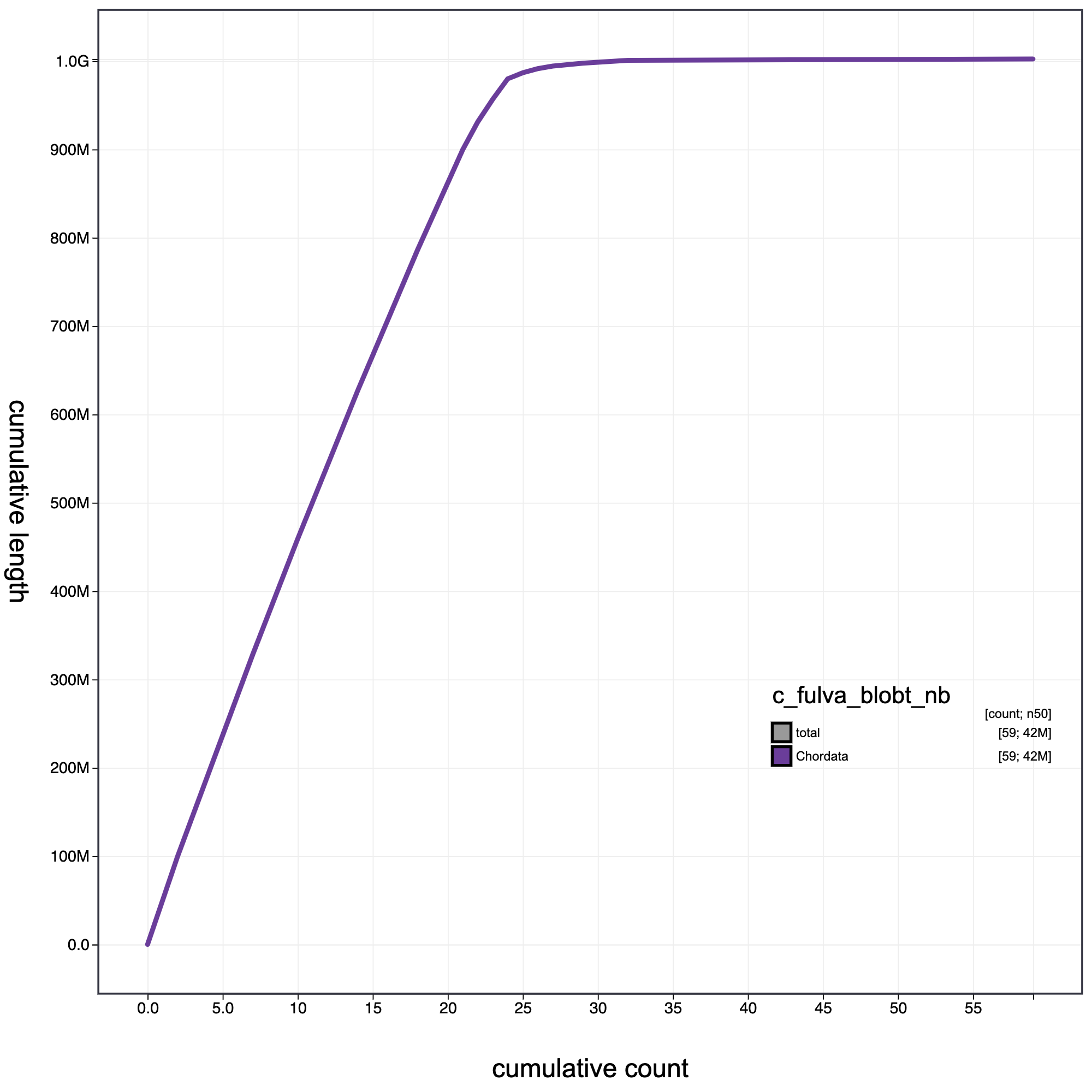
Cumulative record length for c_fulva. The grey line shows cumulative length for all records. Coloured lines show cumulative lengths of records assigned to each phylum using the bestsumorder taxrule.
blob plot
# blob plot
knitr::include_graphics("c_fulva_blob_results/c_fulva_blobt_nb.blob.circle.png")
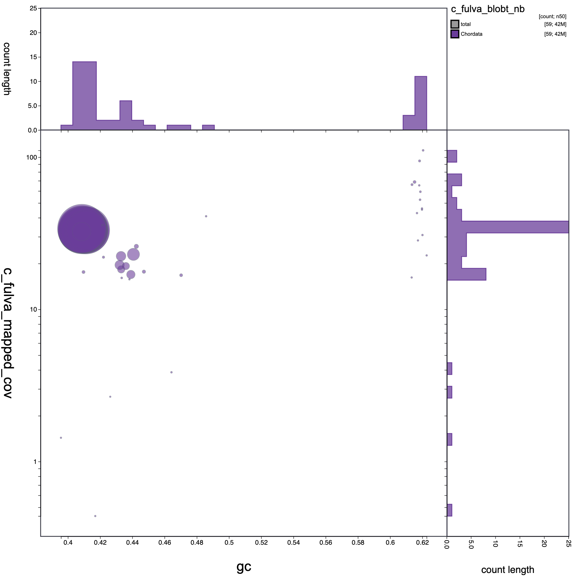
Blob plot of base coverage in p against GC proportion for records in C. fulva assembly. Records are coloured by phylum. Circles are sized in proportion to record length.
blob table with varibles and categories
blob_results<- read.csv("c_fulva_blob_results/8e78fbed-8511-4f58-865d-007ee7d110fc.csv",header = T, sep = ",")
#library(tidyverse)
blob_results<-select(blob_results, -1)
blob_results2<-select(blob_results, 1,8,2,3,7,4,5,6)
blob_results2<-select(blob_results2, -1)
#library(kableExtra)
#blob_results %>% kbl() %>% kable_styling()
#library(DT)
options(scipen = 999)
datatable(blob_results2, rownames = FALSE, width = "100%", colnames = c("ID","GC","Length","Coverage","Phylum", "Class", "Family"),
          caption =
            htmltools::tags$caption(
              style = "caption-side: bottom; text-align: left;",
              "Table: ",
              htmltools::em("blob variables and Categories")),
          extensions = "Buttons",
          options = list(columnDefs =
                           list(list(className = "dt-left", targets = 0)),
                         dom = "Blfrtip", pageLength = 10,
                         lengthMenu = c(10, 20, 40, 70),
                         buttons = c("csv", "copy")))
Chromis multilineata
GenomeScope Results
#GenomeScope Resutls
knitr::include_graphics("c_multilineata_blob_results/linear_plot.png")
#GenomeScope Resutls
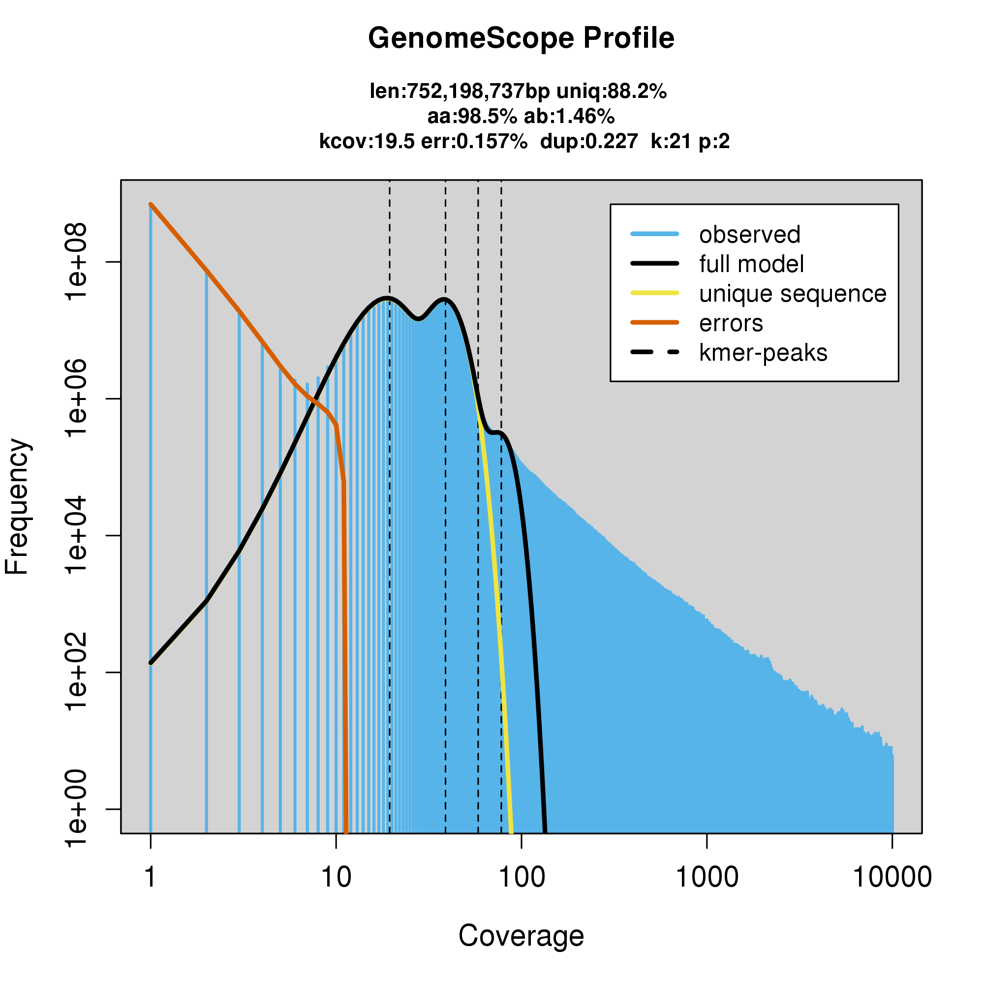
knitr::include_graphics("c_multilineata_blob_results/log_plot.png")
Assembly statistics in a snail plot
#Snail plot/
knitr::include_graphics("c_multilineata_blob_results/c_multilineata_blobt_nb.snail.png")
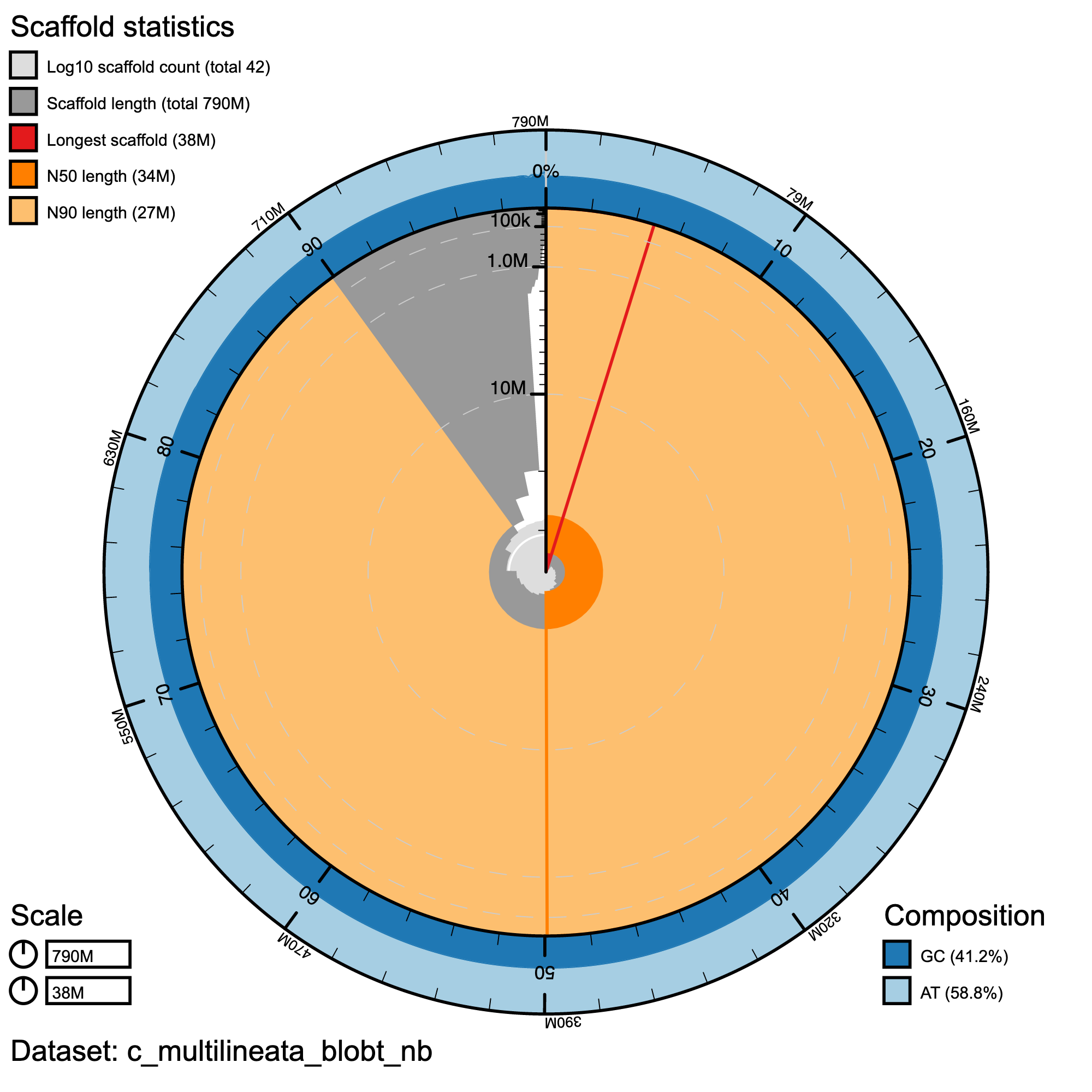
Snail plot summary of assembly statistics for C. multilineata. The main plot is divided into 1,000 size-ordered bins around the circumference with each bin representing 0.1% of the 789,373,866 bp assembly. The distribution of record lengths is shown in dark grey with the plot radius scaled to the longest record present in the assembly (38,245,747 bp, shown in red). Orange and pale-orange arcs show the N50 and N90 record lengths (34,048,903 and 27,186,901 bp), respectively. The pale grey spiral shows the cumulative record count on a log scale with white scale lines showing successive orders of magnitude. The blue and pale-blue area around the outside of the plot shows the distribution of GC, AT and N percentages in the same bins as the inner plot.
Cumulative Plot
#cumulative plot
knitr::include_graphics("c_multilineata_blob_results/c_multilineata_blobt_nb.cumulative.png")
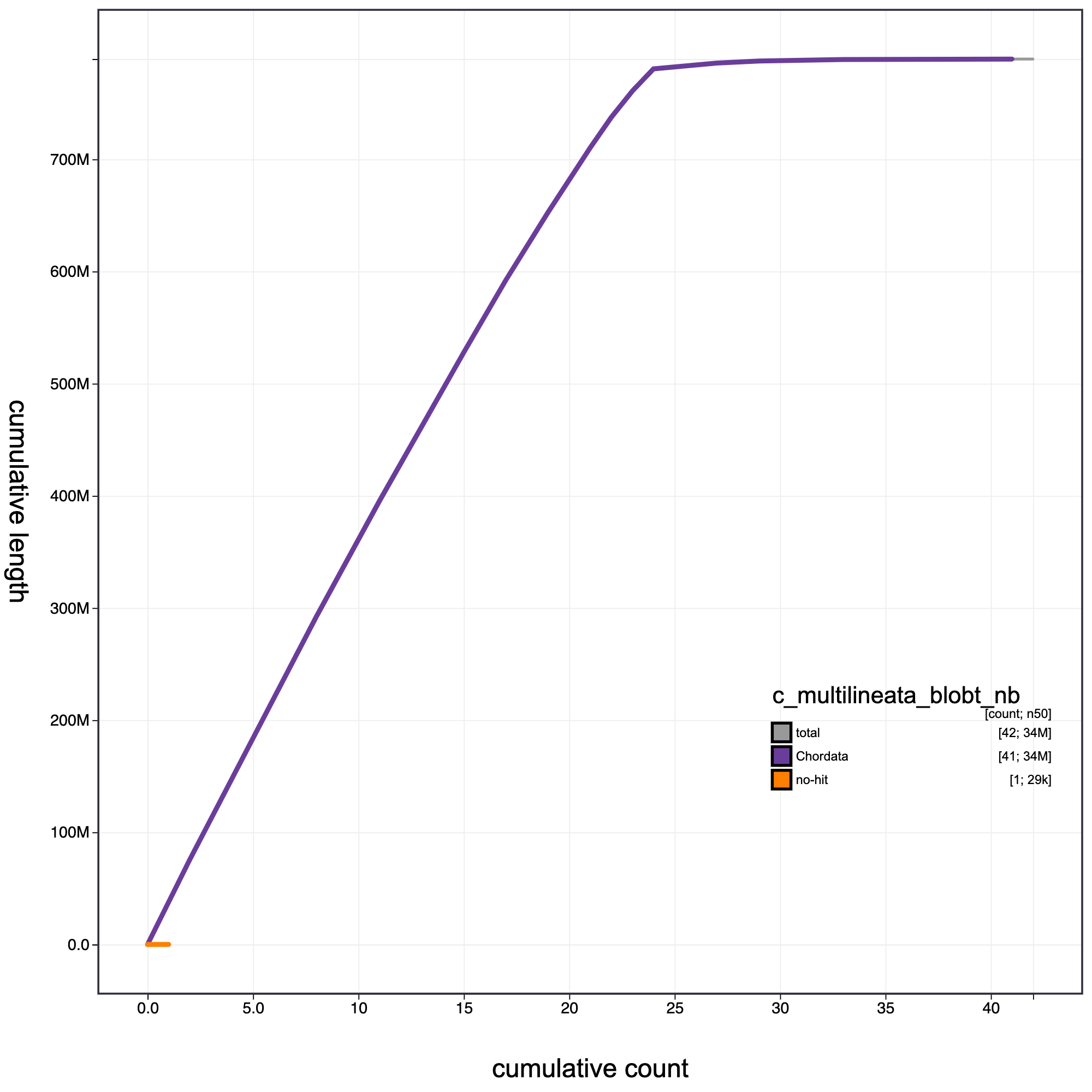
Cumulative record length for C. multilineata assembly. The grey line shows cumulative length for all records. Coloured lines show cumulative lengths of records assigned to each phylum using the bestsumorder taxrule.
blob plot
# blob plot
knitr::include_graphics("c_multilineata_blob_results/c_multilineata_blobt_nb.blob.circle.png")
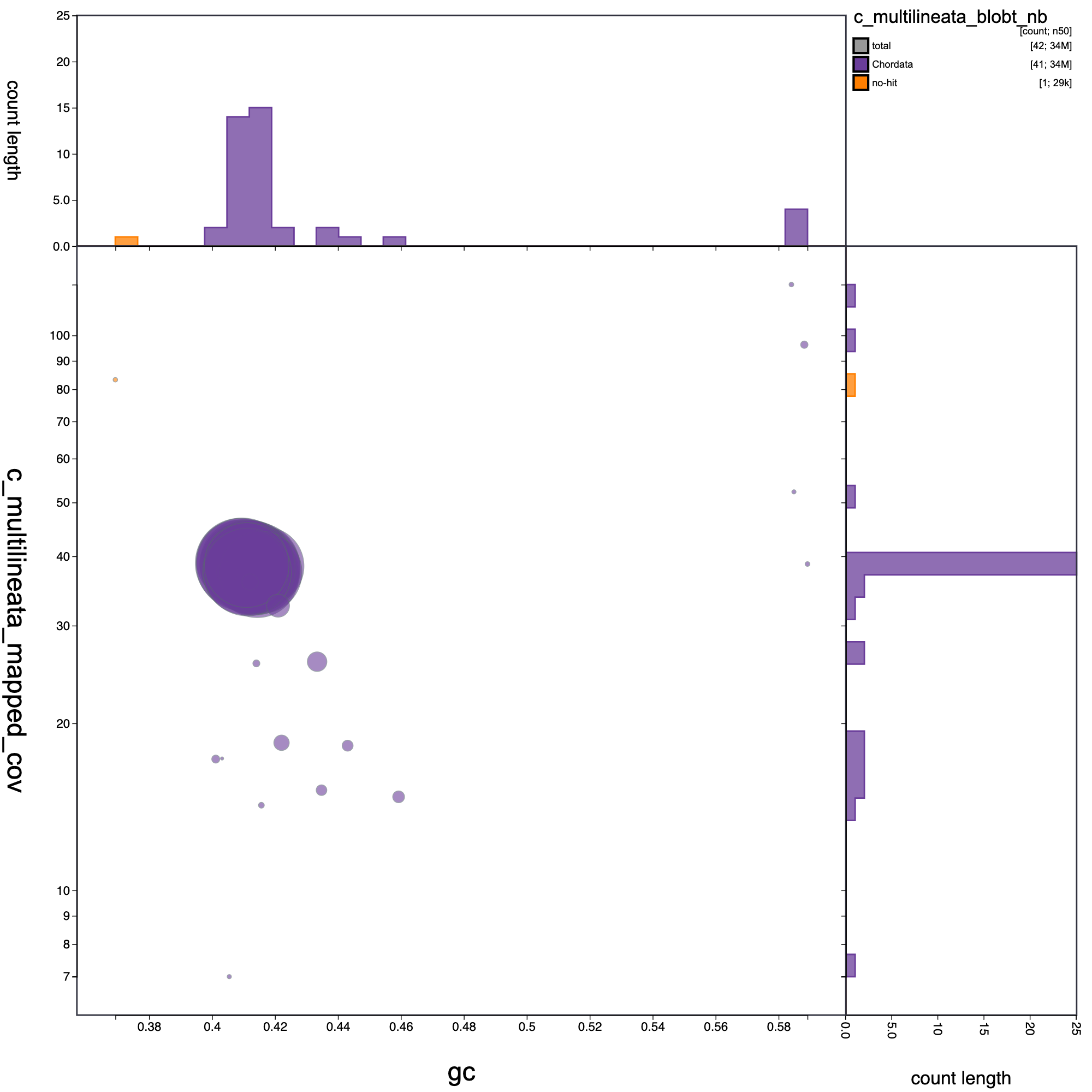
Blob plot of base coverage in p against GC proportion for records in C. multilineata assembly. Records are coloured by phylum. Circles are sized in proportion to record length.
blob table with varibles and categories
blob_results<- read.csv("c_multilineata_blob_results/2a719209-31ee-4daa-bf74-cf1424f52538.csv",header = T, sep = ",")
library(tidyverse)
blob_results<-select(blob_results, -1)
blob_results2<-select(blob_results, 1,8,2,3,7,4,5,6)
blob_results2<-select(blob_results2, -1)
#library(kableExtra)
#blob_results %>% kbl() %>% kable_styling()
#library(DT)
options(scipen = 999)
datatable(blob_results2, rownames = FALSE, width = "100%", colnames = c("ID","GC","Length","Coverage","Phylum", "Class", "Family"),
          caption =
            htmltools::tags$caption(
              style = "caption-side: bottom; text-align: left;",
              "Table: ",
              htmltools::em("blob variables and Categories")),
          extensions = "Buttons",
          options = list(columnDefs =
                           list(list(className = "dt-left", targets = 0)),
                         dom = "Blfrtip", pageLength = 10,
                         lengthMenu = c(10, 20, 40, 70),
                         buttons = c("csv", "copy")))
Chromis atriloba
GenomeScope Results
#GenomeScope Resutls
knitr::include_graphics("c_atrilobata_blob_results/linear_plot.png")
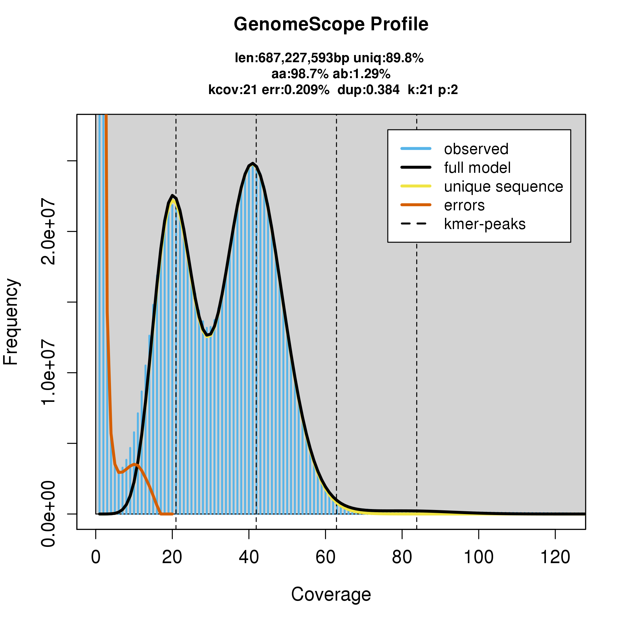
#GenomeScope Resutls
knitr::include_graphics("c_atrilobata_blob_results/log_plot.png")

Assembly statistics in a snail plot
#Snail plot/
knitr::include_graphics("c_atrilobata_blob_results/c_atrilobata_blobt_nb.snail.png")
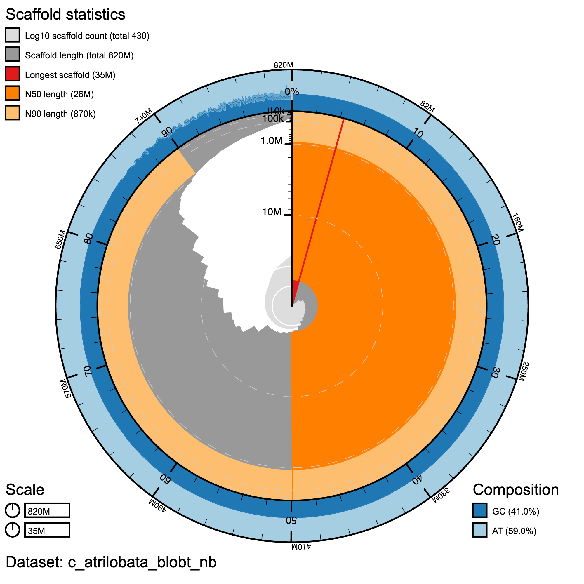
Snail plot summary of assembly statistics for ***C. atrilobata. The main plot is divided into 1,000 size-ordered bins around the circumference with each bin representing 0.1% of the 817,061,737 bp assembly. The distribution of record lengths is shown in dark grey with the plot radius scaled to the longest record present in the assembly (35,142,365 bp, shown in red). Orange and pale-orange arcs show the N50 and N90 record lengths (26,205,343 and 869,398 bp), respectively. The pale grey spiral shows the cumulative record count on a log scale with white scale lines showing successive orders of magnitude. The blue and pale-blue area around the outside of the plot shows the distribution of GC, AT and N percentages in the same bins as the inner plot.
Cumulative Plot
#cumulative plot
knitr::include_graphics("c_atrilobata_blob_results/c_atrilobata_blobt_nb.cumulative.png")
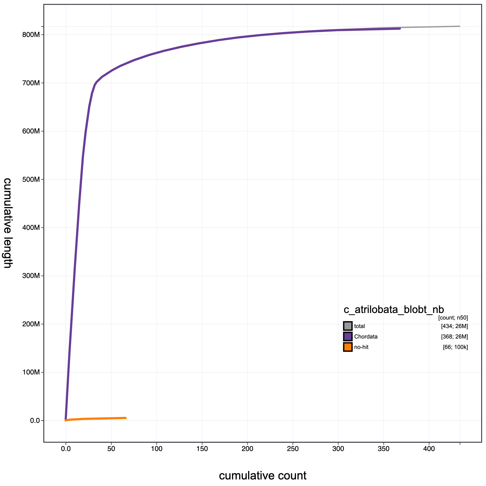
Cumulative record length for C. atrilobata assembly. The grey line shows cumulative length for all records. Coloured lines show cumulative lengths of records assigned to each phylum using the bestsumorder taxrule.
blob plot
# blob plot
knitr::include_graphics("c_atrilobata_blob_results/c_atrilobata_blobt_nb.blob.circle.png")
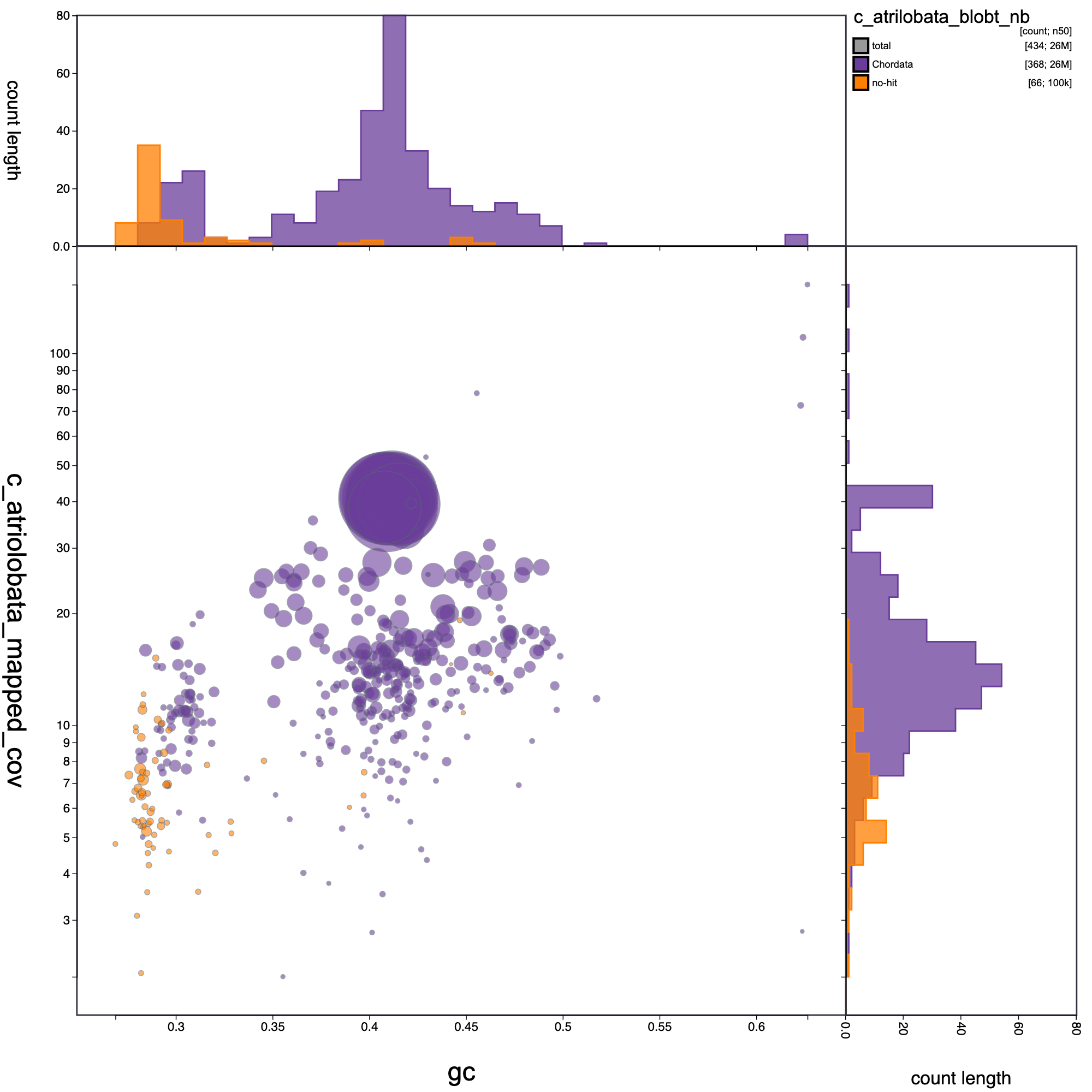
Blob plot of base coverage in p against GC proportion for records in C. atrilobata assembly. Records are coloured by phylum. Circles are sized in proportion to record length.
blob table with varibles and categories
blob_results<- read.csv("c_atrilobata_blob_results/2ba4906a-f4e2-4662-ab36-67bcde2f380f.csv",header = T, sep = ",")
library(tidyverse)
blob_results<-select(blob_results, -1)
blob_results2<-select(blob_results, 1,8,2,3,7,4,5,6)
blob_results2<-select(blob_results2, -1)
#library(kableExtra)
#blob_results %>% kbl() %>% kable_styling()
#library(DT)
options(scipen = 999)
datatable(blob_results2, rownames = FALSE, width = "100%", colnames = c("ID","GC","Length","Coverage","Phylum", "Class", "Family"),
          caption =
            htmltools::tags$caption(
              style = "caption-side: bottom; text-align: left;",
              "Table: ",
              htmltools::em("blob variables and Categories")),
          extensions = "Buttons",
          options = list(columnDefs =
                           list(list(className = "dt-left", targets = 0)),
                         dom = "Blfrtip", pageLength = 10,
                         lengthMenu = c(10, 20, 40, 70),
                         buttons = c("csv", "copy")))
Chromis cyanea
GenomeScope Results
#GenomeScope Resutls
knitr::include_graphics("c_cynea_blob_results/linear_plot.png")
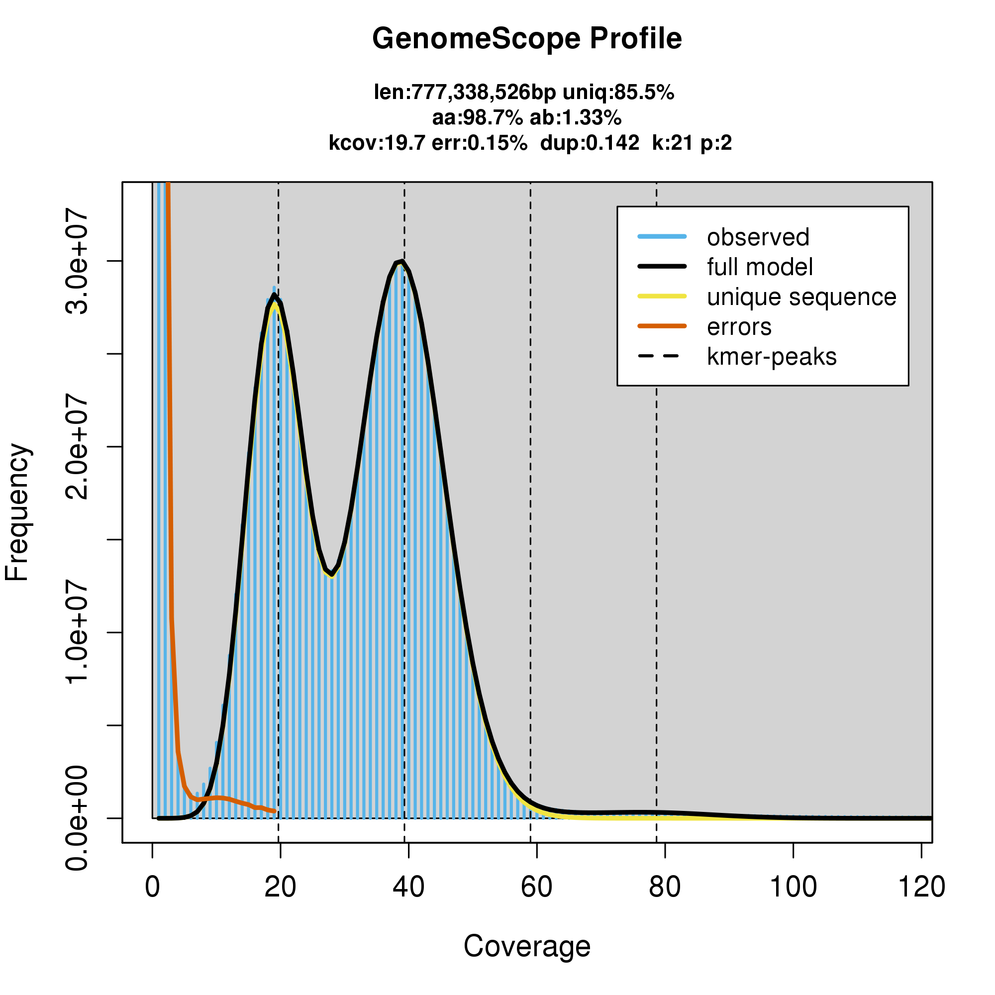
#GenomeScope Resutls
knitr::include_graphics("c_cynea_blob_results/log_plot.png")

Assembly statistics in a snail plot
#Snail plot/
knitr::include_graphics("c_cynea_blob_results/c_cyanea_blobtnb.snail.png")
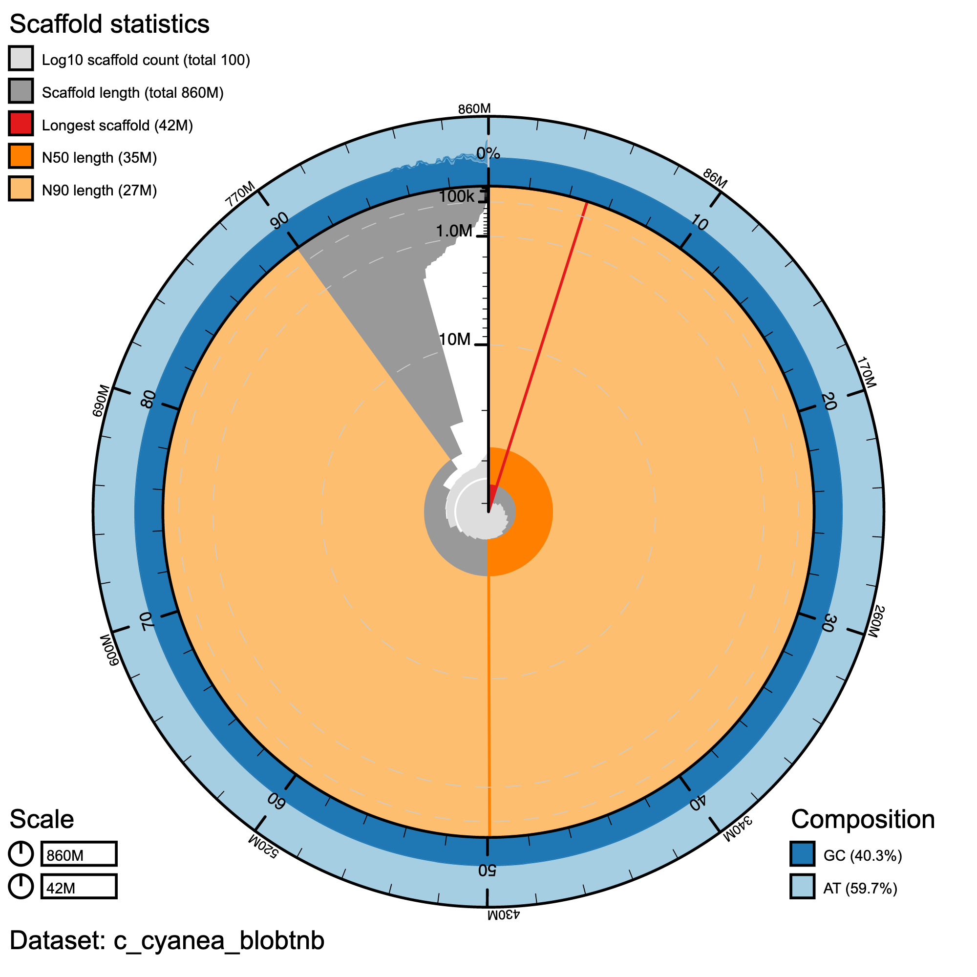
Snail plot summary of assembly statistics for C._cyanea. The main plot is divided into 1,000 size-ordered bins around the circumference with each bin representing 0.1% of the 858,680,933 bp assembly. The distribution of record lengths is shown in dark grey with the plot radius scaled to the longest record present in the assembly (42,133,999 bp, shown in red). Orange and pale-orange arcs show the N50 and N90 record lengths (35,016,054 and 27,092,967 bp), respectively. The pale grey spiral shows the cumulative record count on a log scale with white scale lines showing successive orders of magnitude. The blue and pale-blue area around the outside of the plot shows the distribution of GC, AT and N percentages in the same bins as the inner plot.
Cumulative Plot
#cumulative plot
knitr::include_graphics("c_cynea_blob_results/c_cyanea_blobtnb.cumulative.png")
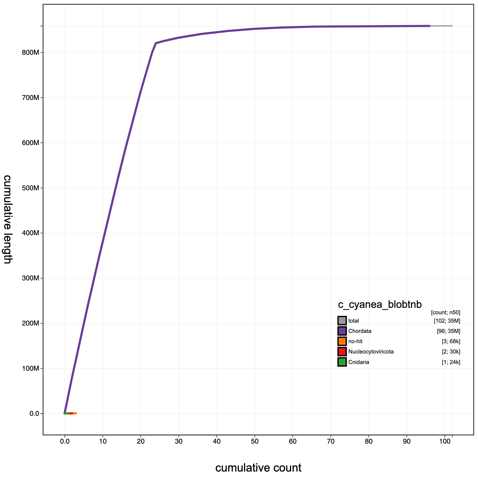
Cumulative record length for C. cyanea assembly.The grey line shows cumulative length for all records. Coloured lines show cumulative lengths of records assigned to each phylum using the bestsumorder taxrule.
blob plot
# blob plot
knitr::include_graphics("c_cynea_blob_results/c_cyanea_blobtnb.blob.circle.png")
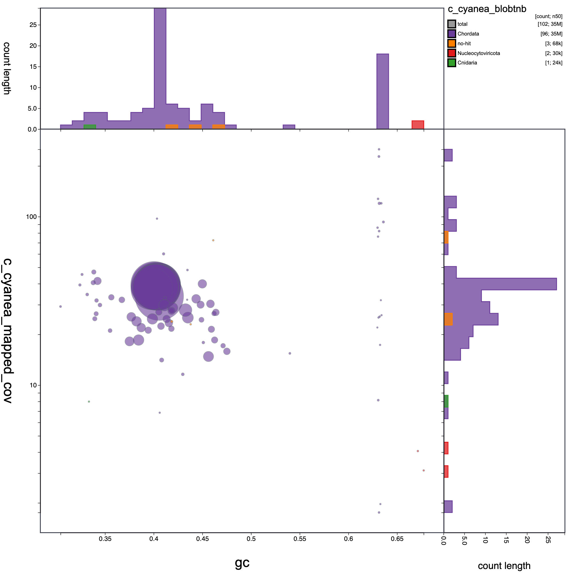
Blob plot of base coverage in p against GC proportion for records in C. cyanea assembly. Records are coloured by phylum. Circles are sized in proportion to record length.
blob table with varibles and categories
blob_results<- read.csv("c_cynea_blob_results/cd6a4b7f-9e60-40a2-b3e9-cea95e3f60ee.csv",header = T, sep = ",")
#library(tidyverse)
blob_results<-select(blob_results, -1)
blob_results2<-select(blob_results, 1,8,2,3,7,4,5,6)
blob_results2<-select(blob_results2, -1)
#library(kableExtra)
#blob_results %>% kbl() %>% kable_styling()
#library(DT)
options(scipen = 999)
datatable(blob_results2, rownames = FALSE, width = "100%", colnames = c("ID","GC","Length","Coverage","Phylum", "Class", "Family"),
          caption =
            htmltools::tags$caption(
              style = "caption-side: bottom; text-align: left;",
              "Table: ",
              htmltools::em("blob variables and Categories")),
          extensions = "Buttons",
          options = list(columnDefs =
                           list(list(className = "dt-left", targets = 0)),
                         dom = "Blfrtip", pageLength = 10,
                         lengthMenu = c(10, 20, 40, 70),
                         buttons = c("csv", "copy")))
Abudefduf troshelii
GenomeScope Results
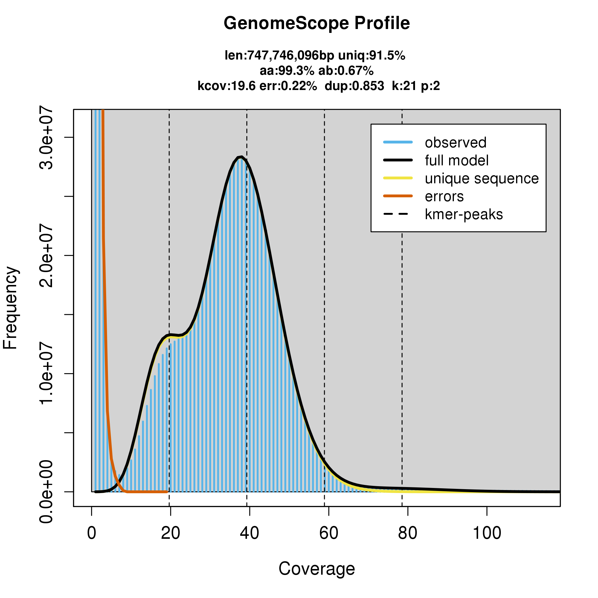
#GenomeScope Resutls
knitr::include_graphics("a_troshelii_blob_results/linear_plot.png")
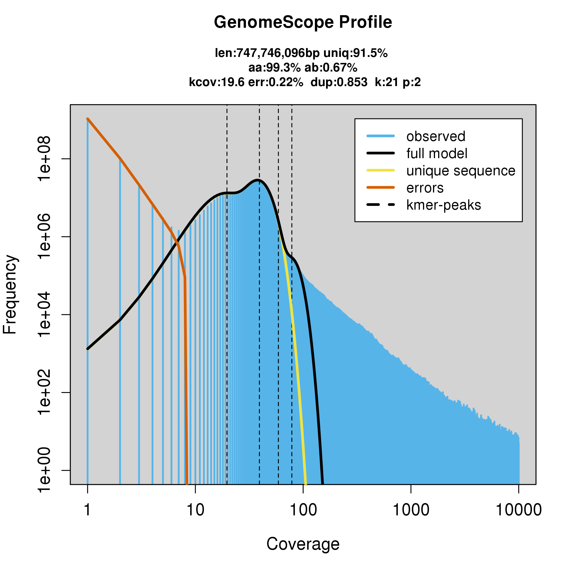
#GenomeScope Resutls
knitr::include_graphics("a_troshelii_blob_results/log_plot.png")
Assembly statistics in a snail plot
#Snail plot/
knitr::include_graphics("a_troshelii_blob_results/a_troshelii_blobt_nb.snail.png")
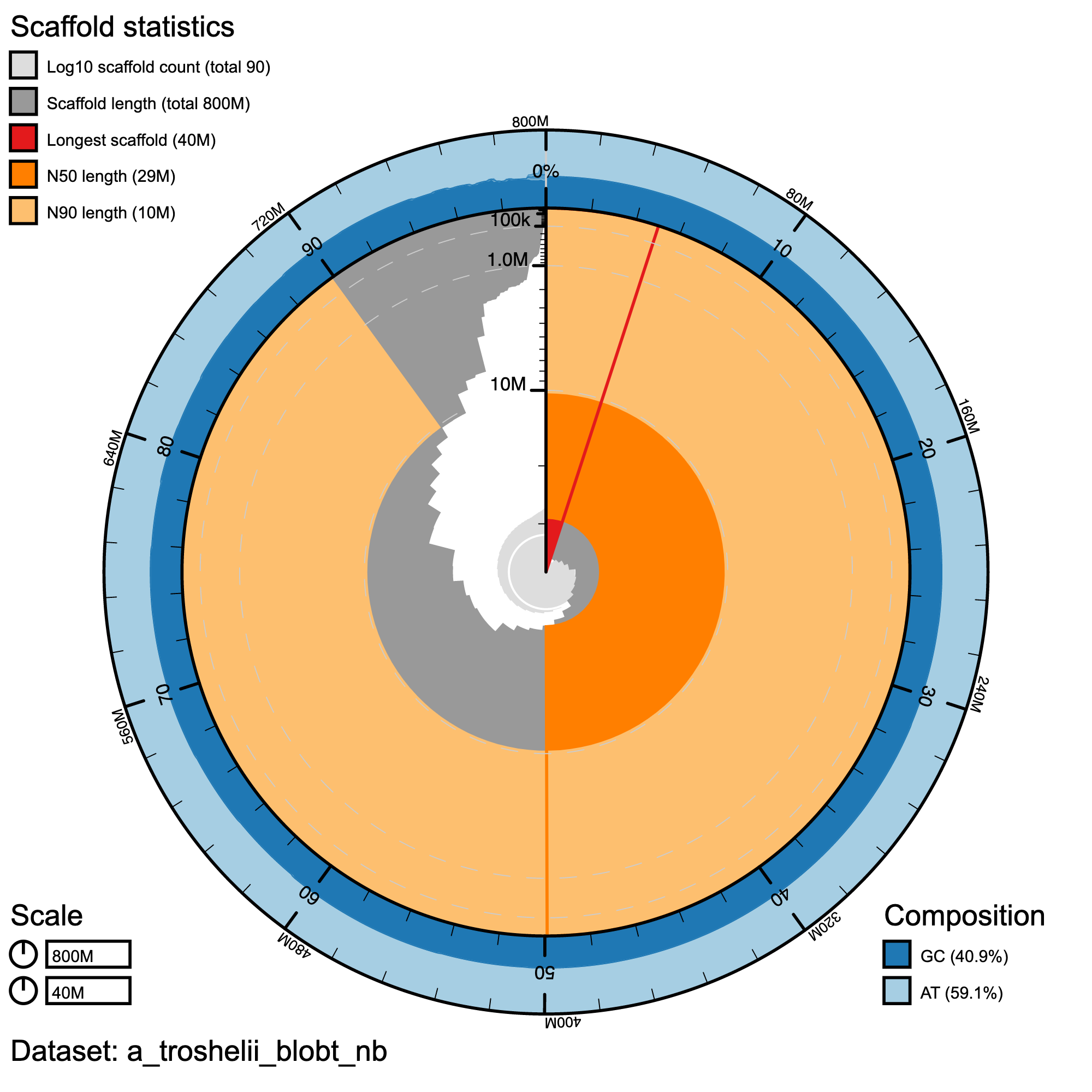
Snail plot summary of assembly statistics for A_troshelii. The main plot is divided into 1,000 size-ordered bins around the circumference with each bin representing 0.1% of the 796,160,303 bp assembly. The distribution of record lengths is shown in dark grey with the plot radius scaled to the longest record present in the assembly (39,846,712 bp, shown in red). Orange and pale-orange arcs show the N50 and N90 record lengths (28,775,316 and 10,326,087 bp), respectively. The pale grey spiral shows the cumulative record count on a log scale with white scale lines showing successive orders of magnitude. The blue and pale-blue area around the outside of the plot shows the distribution of GC, AT and N percentages in the same bins as the inner plot.
Cumulative Plot
#cumulative plot
knitr::include_graphics("a_troshelii_blob_results/a_troshelii_blobt_nb.cumulative.png")
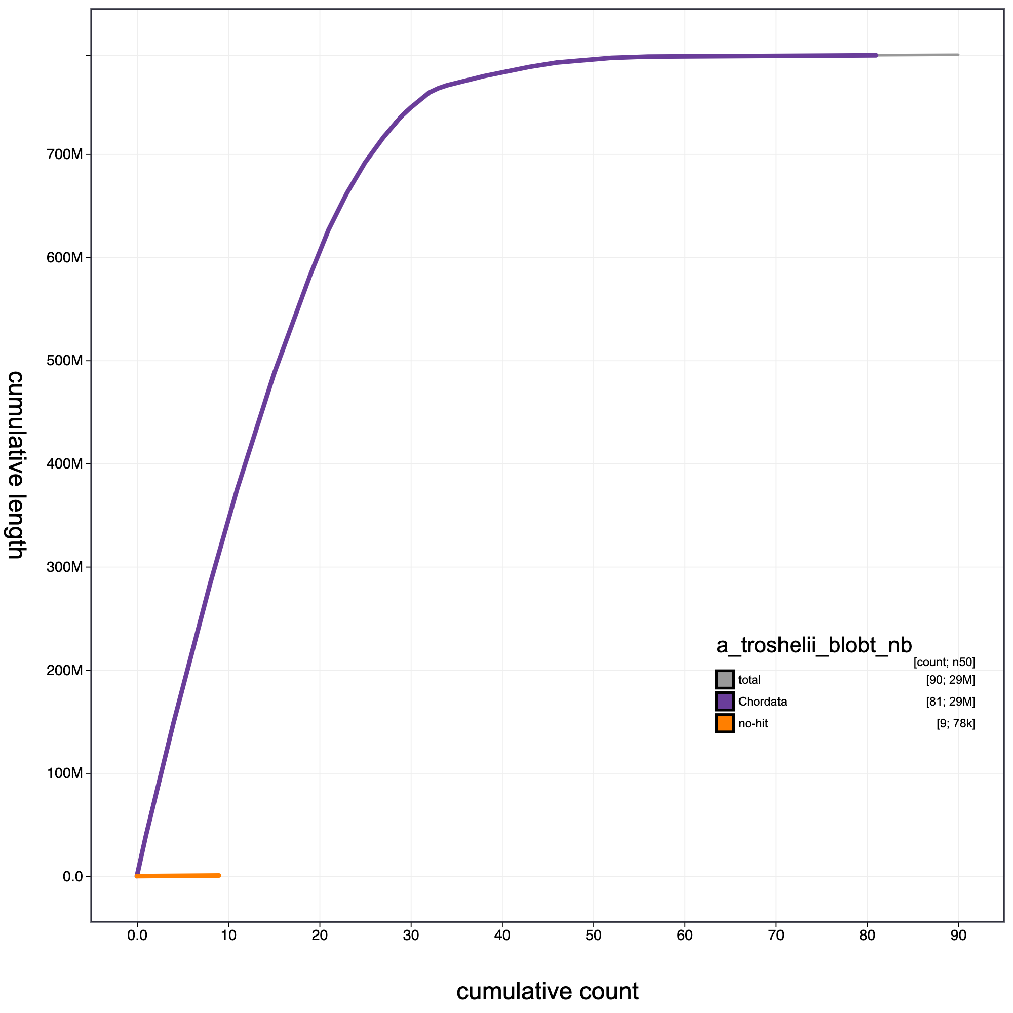
Cumulative record length for A._troshelii assembly .The grey line shows cumulative length for all records. Coloured lines show cumulative lengths of records assigned to each phylum using the bestsumorder taxrule.
blob plot
# blob plot
knitr::include_graphics("a_troshelii_blob_results/a_troshelii_blobt_nb.blob.circle.png")
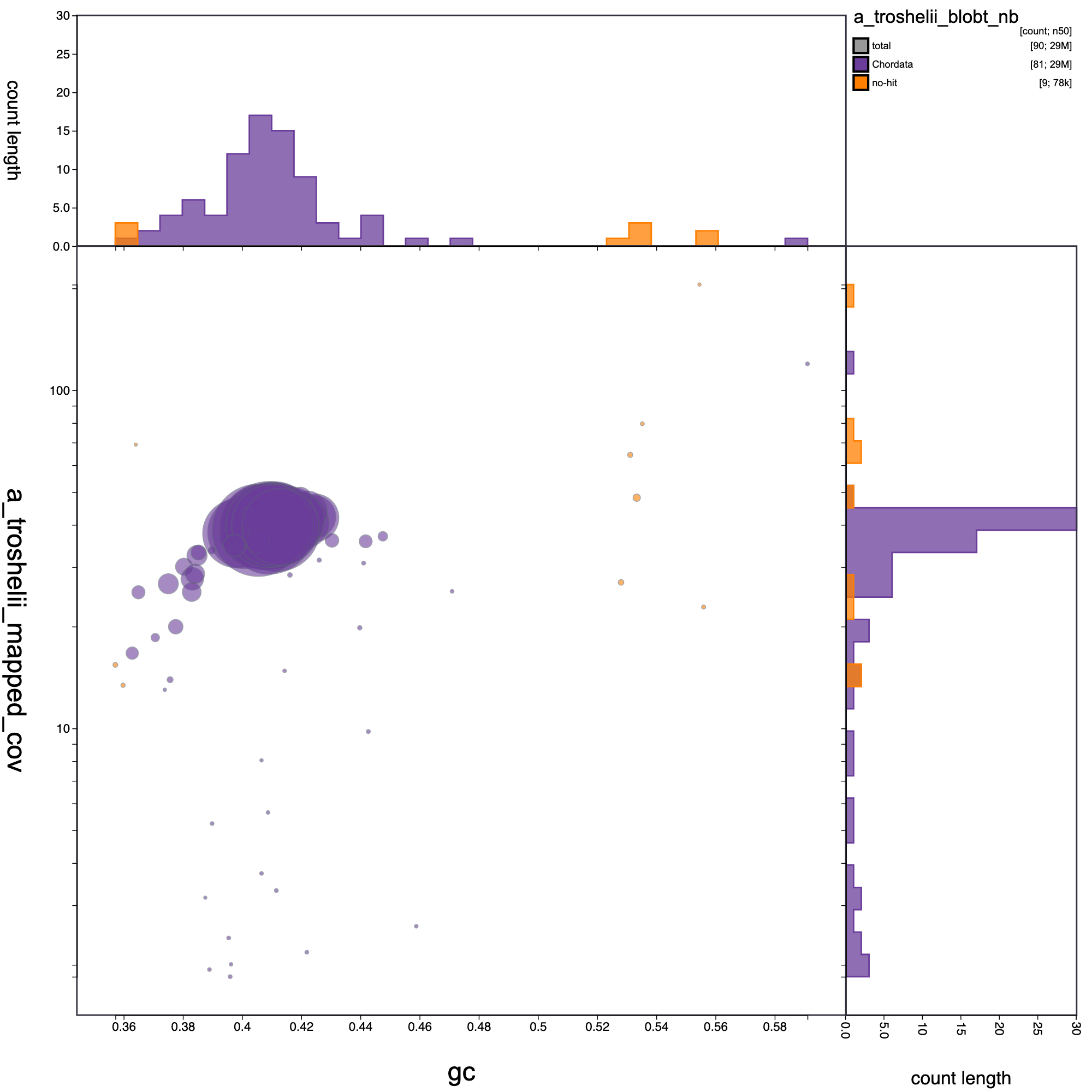
Blob plot of base coverage in p against GC proportion for records in A. troshelii assembly. Records are coloured by phylum. Circles are sized in proportion to record length.
blob table with varibles and categories
blob_results<- read.csv("a_troshelii_blob_results/00ff4f5e-bd43-4c48-b4c8-9e2e9b971300.csv",header = T, sep = ",")
#library(tidyverse)
blob_results<-select(blob_results, -1)
blob_results2<-select(blob_results, 1,8,2,3,7,4,5,6)
blob_results2<-select(blob_results2, -1)
#library(kableExtra)
#blob_results %>% kbl() %>% kable_styling()
#library(DT)
options(scipen = 999)
datatable(blob_results2, rownames = FALSE, width = "100%", colnames = c("ID","GC","Length","Coverage","Phylum", "Class", "Family"),
          caption =
            htmltools::tags$caption(
              style = "caption-side: bottom; text-align: left;",
              "Table: ",
              htmltools::em("blob variables and Categories")),
          extensions = "Buttons",
          options = list(columnDefs =
                           list(list(className = "dt-left", targets = 0)),
                         dom = "Blfrtip", pageLength = 10,
                         lengthMenu = c(10, 20, 40, 70),
                         buttons = c("csv", "copy")))